Viewing images
In this tutorial, we’ll go over the steps needed to load images in Horta and view them.
HortaCloud-focused
This tutorial is focused on HortaCloud. However, most of it applies to the desktop version of Horta as well. If you can launch Horta on the desktop, and you see data in the Data Explorer, you should be able to follow most of the other steps of the tutorial.Prerequisites
- You should be able to log into HortaCloud and launch the Horta application, as detailed in the previous tutorial.
- Your HortaCloud instance should have access to the Janelia MouseLight data on Amazon AWS S3.
- If not, you should have access to some similar data in your HortaCloud instance.
Steps
Start the Horta Application
Launch the Horta application. See the previous tutorial “Logging in” for more detail.
Locate and examine data in the Data Explorer
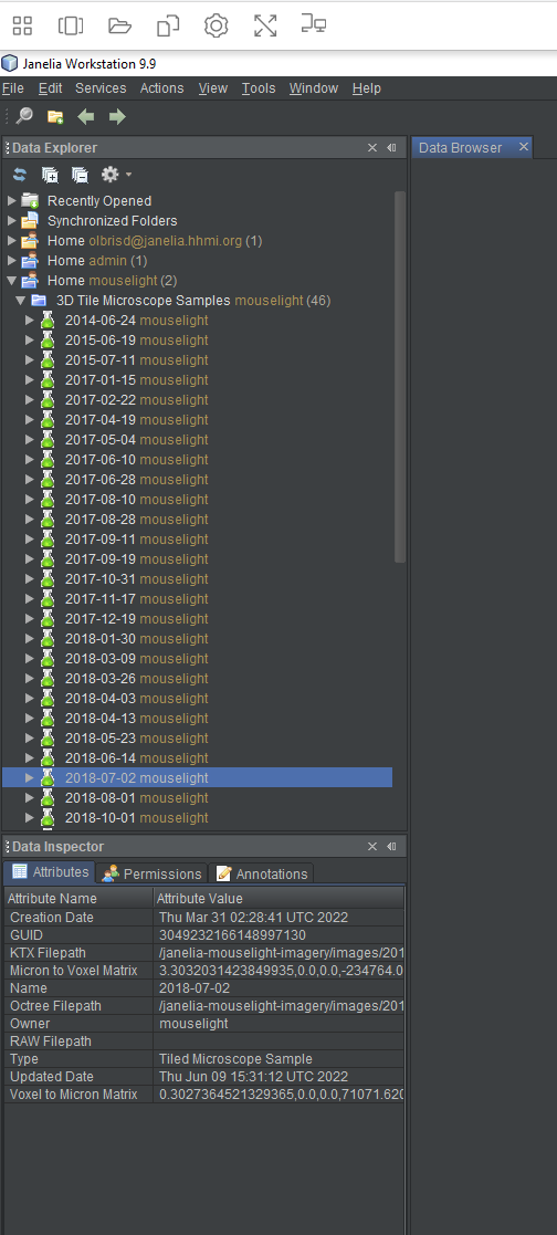
The “Data Explorer”, which appears by default in the upper left panel of Horta, shows a representation of all the data in Horta that you are allowed to see. This data is organized in folders, both created by the system and created by users. The exact list of folder you see will differ depending on which data you have permission to see.
Click on the triangle to the left of the folder named Home with the owner mouselight, which appears immediately to the right of the folder name, in yellow. This will open the folder to show its contents.
Click on the triangle to the left of the “3D Tile Microscope Samples” folder, also owned by mouselight. You will see a long list of samples, indicated by a green flask icon. Each of these sample represents a group of image files on disk or in an AWS S3 bucket.
For this tutorial, we’re going to look at one of the Janelia Mouse Light samples, the 2018-07-02 sample. Scroll down the list of samples until you see it. Left-click on the sample to select it. You will see information appear in the “Data Inspector”, located just below the Data Explorer.
The three tabs of the Data Inspector each show information about the sample. The “Attributes” tab contains typical metadata like name, creation/modification date, and globally unique identifier (GUID). It also shows the sample’s owner and the location of the image files that belong to the sample. The “Permissions” tab shows which users or groups can read or write to the data. There’s also a button which allows someone to grant permissions to other users to see or edit the data. The third tab, “Annotations”, is not used by Horta and is only used with other tools in the desktop workstation client.
Open a sample in Horta
Now that we’ve located the 2018-07-02 sample, it’s time to open it in Horta.
Do one of two things:
- Right-click the sample, and choose “Open in Horta”.
- Left-click the sample to select it; then choose
Horta>Open in Hortafrom theActionsmenu.
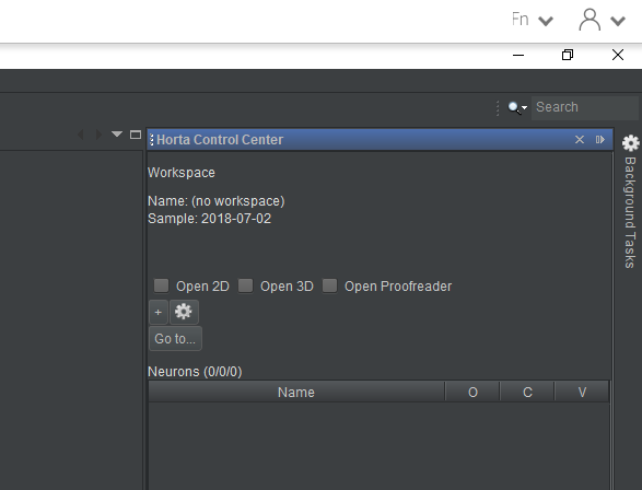
At this point, not a lot will visibly happen. When you open a sample in Horta, all that happens is that the dataset’s metadata is loaded into the application. The images themselves are not yet loaded. You will see that in the “Horta Control Center” panel at right, near the top below the “WORKSPACE” heading, the “Sample” field will now show the name “2018-07-02”. That’s all (screenshot below). In the next tutorial (“Tracing neurons”), we’ll see that opening a workspace in Horta populates much more information in the UI. The “Concepts” section of the documentation has more information on the difference between samples and workspaces.
Open the Horta 3D window
It’s time to finally look at some images. For this demonstration, we’ll start with the 3D images. Near the top of the Horta Control Center, under the “VIEWS” heading, find the checkbox labeled “Open 3D”. Click it so it’s checked.
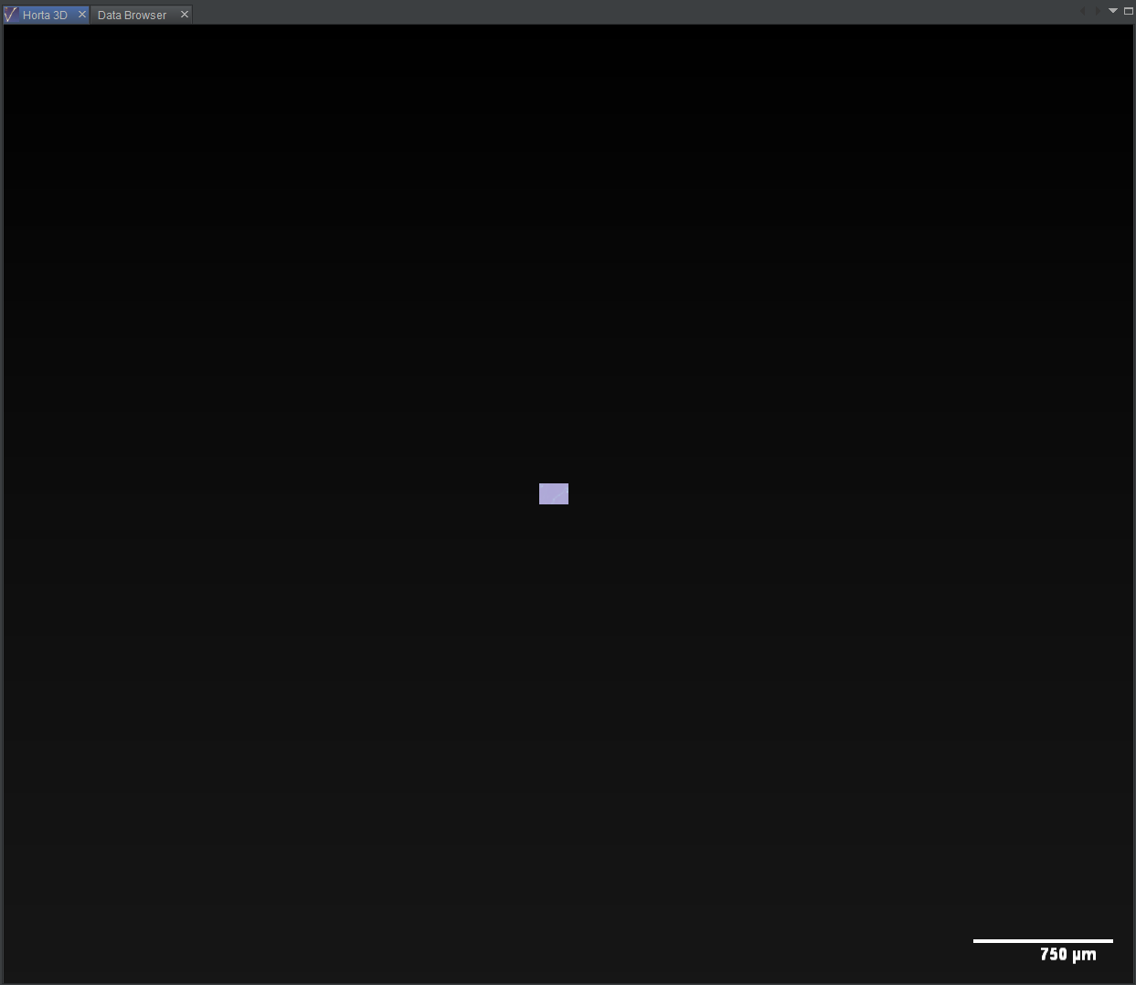
You will see a window tab titled “Horta 3D” open in the center panel. The first 3D images will also load. Initially, it’ll be underwhelming. Probably you’ll see one small bright rectangle in the center of the screen. In the next section, we’ll see how to adjust the color. For now, if you left-click in the 3D window, more data will load to cover most of the window.
Explore the data in 3D
Adjust colors
The default color settings are not good; in general, the data will appear to be a washed out bright, light blue/purple. In order to adjust the color, first we need to go to the “Windows” menu and choose Horta > Color Sliders.
Often when the sliders are first opened, their panel will not be the correct height. You can adjust this. Like other panels in Horta, the color slider panel may be resized and docked or undocked from the main window as you like.
Also, when the color sliders are first opened, often the 3D image will be redrawn, or potentially not drawn at all. If this occurs, left-click in the 3D window to trigger a redraw.
Even though the data only has two channels (a signal channel and a reference channel), you’ll see three sliders. The third blue slider has a specialized use that we’re not going to cover in this tutorial. Click the eye next to the blue slider, and the blue channel will be hidden.
In practice, you will likely spend a lot of time tuning the color settings so the desired biological structures are most visible. For this tutorial, we’ll cover a few simple steps to make the data more visible:
- First, you can optionally display the numeric values of the sliders by clicking the
#button at the far right of each color slider, just before the color swatch. This is useful if you want to adjust values finely. It’s also useful to communicate the values to another user. But note if you want to import or export all of the color settings at once, you can do so using those options on the gear menu in the lower right corner of the color slider panel. - Click the eye icon to the left of the top, green slider. This turns the green channel data invisible.
- Now drag the leftmost slider of the middle, purple slider to the right. Do this until the blocky, purple background of the image tiles disappears and you can see the purple outline of the brain. For this data, you’ll be dragging the slider until it’s midway between the left edge and the center lock icon below the sliders. If you have the numbers showing, set “Min” to around 15600.
- Now do it again for green. Click the eye next to the green slider to show the green channel, and the eye next to the purple channel to hide it. Drag the leftmost slide of the green bar until, again, the blocky background disappears and the brain outline is visible. For this data, try setting it a bit to the left of the left purple slider. That’s around a value of 12200 for “Min”.
- Click the eye next to the purple slide so both data channels are visible again.
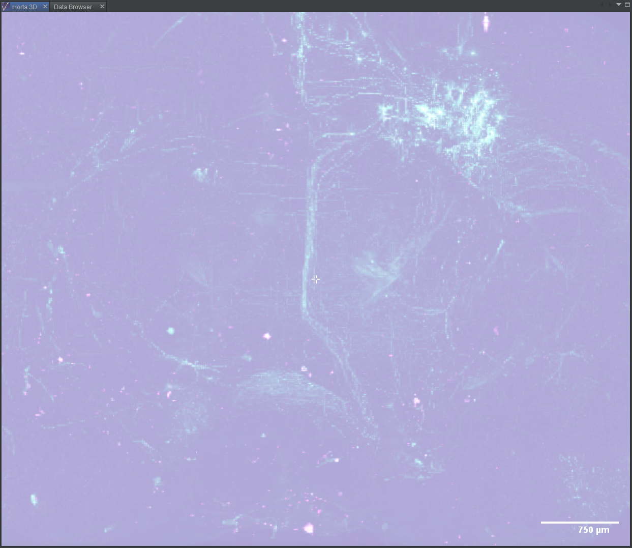
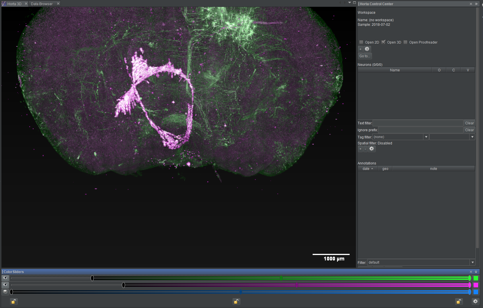
At this point (screenshot below), the labeled neurons, though, stand out in green against the purple background. Feel free to experiment with the other sliders. It’s a matter of personal preference. Some tracers prefer to adjust the settings until the background is nearly invisible, so that the neuron signal is prominent, even if dim.
Note: Color settings are not saved for samples! In the next tutorial, we’ll see how these settings are saved in workspaces.
Pan, zoom, rotate
Navigating the 3D data is done using the mouse.
To navigate in space (pan):
- left-click to center on a location
- left-drag to move the image in the view plane
- as you navigate, images will be loaded and unloaded
To zoom in and out:
- use the scroll wheel to zoom in or out; as you zoom, higher or lower resolutions images will be loaded
- note that as you zoom in, you will see less and less of the thickness of the brain; that is, the displayed data will come from a projection depth that is smaller, allowing you to more clearly isolate smaller structures as you zoom in
To rotate in 3D:
- middle-click and drag, or hold down the shift key and left-click and drag; the cursor will change to two curved arrows, and the image will rotate in three dimensions
Open the Horta 2D window
HortaCloud
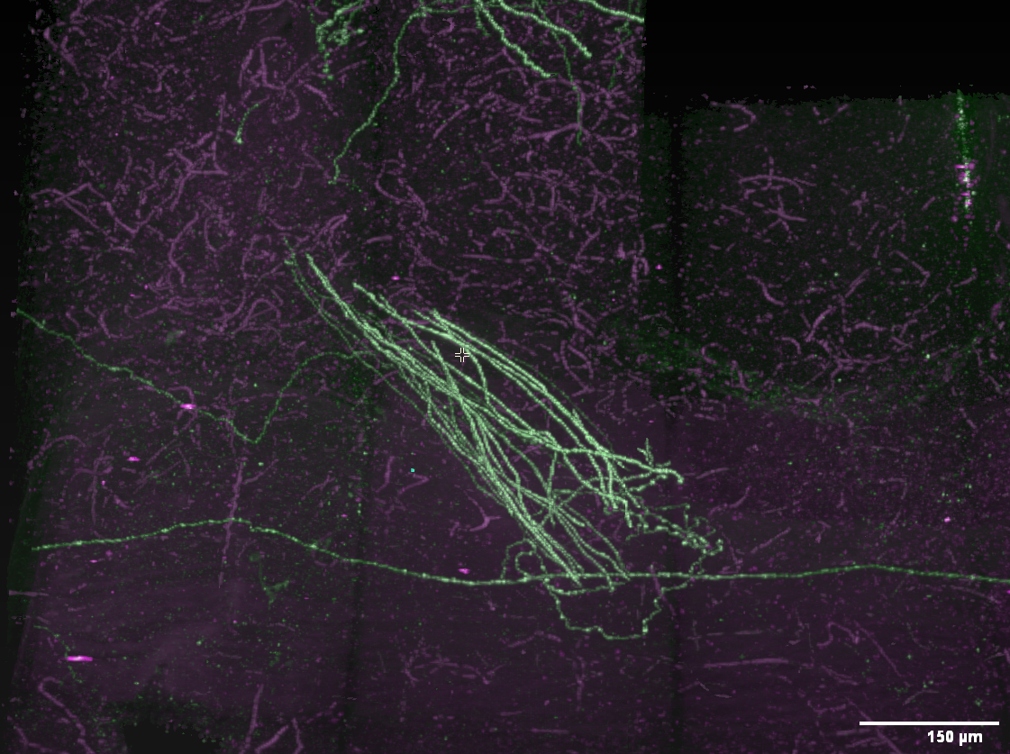
Note that HortaCloud does not store high-resolution 2D images! When you zoom in, the images will be blurry.
In the Horta desktop application, when you zoom in, higher-resolution images will automatically be loaded.
Loading the 2D images is done just like for 3D. Near the top of the Horta Control Center, in the “VIEWS” section, find the checkbox labeled “Open 2D”. Click it so it’s checked.
You will see a window tab titled “Horta 2D” open in the center panel. The first 2D images will also load.
Explore the data in 2D
Adjust colors
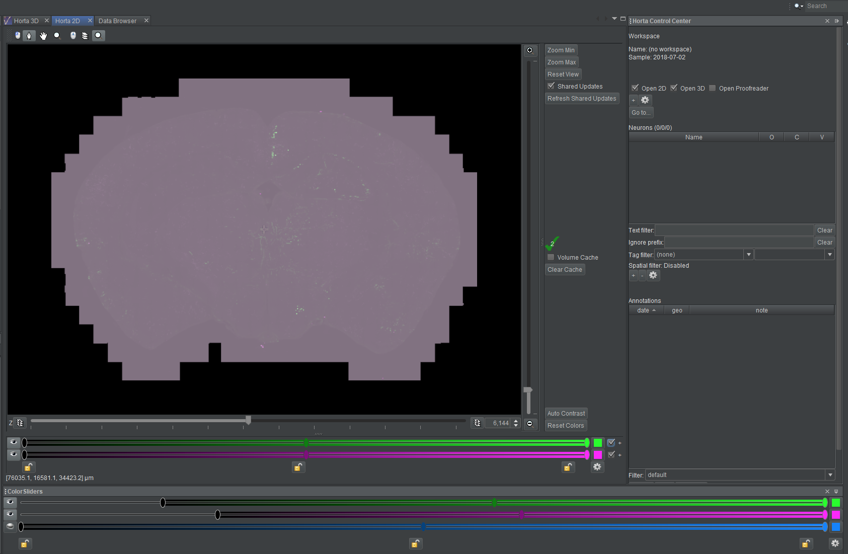
As with 3D, the default color settings are almost never useful, and we’ll quickly adjust them to make the data more visible. In practice, you will likely spend a lot of time tuning the color settings so the desired biological structures are most visible.
The colors of the two data channels are controlled by the sliders and buttons at the bottom of the middle panel in the “Horta 2D” tab. They are distinct from the sliders used to adjust the 3D colors.
NOTE: Sometimes the color slider do not draw correctly when the sample initially opens in 2D. If this is the case, you will see two small checkboxes and two small plus signs at the right of the empty area below the 2D image. Toggle either on of the check boxes off and on, and the sliders should redraw.
Here are the steps to make some minimal adjustments to the colors:
- As before, you can optionally display the numeric values of the sliders by clicking the
#button at the far right of each color slider - Click the eye icon to the left of the top, green slider. This turns the green channel data invisible.
- Now drag the leftmost slider of the lower, purple slider to the right. Do this until the blocky, purple background of the image tiles disappears and you can see the purple outline of the brain. For this data, you’ll be dragging the slider until it’s midway between the left edge and the center lock icon below the sliders. Try a value of “Min” = 15200.
- Now do it again for green. Click the eye next to the green slider to show the green channel, and the eye next to the purple channel to hide it. Drag the leftmost slide of the green bar until, again, the blocky background disappears and the brain outline is visible. For this data, try a location just to the left of the middle purple slider. Try “Min” = 11800.
- Click the eye next to the purple slide so both data channels are visible again.
At this point (screenshot), the labeled neurons stand out in green against the purple background. Feel free to experiment with the other sliders. Again, it’s a matter of preference, your data, and your display, among other things.
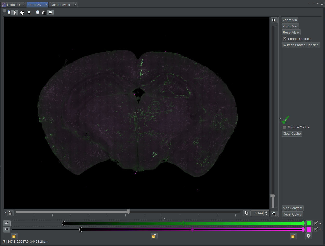
Note: Color settings are not saved for samples! In the next tutorial, we’ll see how these settings are saved in workspaces.
Pan, scroll through z, zoom
Navigating the 2D data is done using the mouse.
To navigate in the x-y plane, you can:
- double-left-click on any location to center the view on that point
- middle-click and drag to pan the image to any location
To navigate along the z-axis, you can:
- use the scroll wheel to change the visible plane
- drag the horizontal slider below the 2D view to change the visible plane
- change the plane number visible in the plane number box to the right of the plane slider by either typing a plane number in the box, or by clicking the up and down arrows in the box
To zoom the image:
- hold down the shift key and spin the scroll wheel
- drag the vertical slider to the right of the 2D view
- remember, HortaCloud does not has high-resolution 2D images; when you zoom in, it will be blurry!
x, y, z locations
Status bars
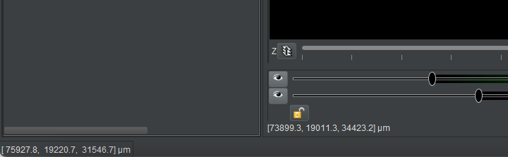
As you move the mouse cursor in either the 2D or 3D windows, you will see the x, y, z location of the cursor displayed in the status bars.
- in 3D, the status bar is at the very bottom of the Horta application window
- in 2D, the status bar is at the bottom of the 2D window; the 3D status bar in this case is not accurate, and it does not update
- in both cases, the
x, y, zlocation is given in microns (µm), as a floating-point number
The screenshot below shows both status bars, with the 3D bar at the bottom and the 2D bar above it.
Copying location values
You can copy the the current x, y, z location to the clipboard by right-clicking in the view.
- in 3D, right-click and choose “Copy Micron Location to Clipboard”
- in 2D, right-click and choose “Copy Micron Coords to Clipboard”
- in both cases, the copied text has the following form:
[68665.88,48154.89,26670.117]- this is convenient for pasting into eg Matlab or Python
- (HortaCloud) see the “AppStream Basics” section in this documentation for how to transfer the data from AppStream’s clipboard to your local system’s clipboard
Go to point
If you know the x, y, z location you’d like to navigate to, and that data is on the clipboard, click the “Go to location…” button that appears in the “VIEWS” section in the Horta Control Center. Paste in the data from the clipboard and click “OK”. Both the 2D and 3D views will navigate to put that point at the center of the view without changing the zoom level.
Details:
- the values should be in microns
- you can paste in
x, y, zcoordinates or justx, y; in the latter case, the currentzvalue will not change - any brackets or commas will be removed
- thus you can copy and paste from Horta, or from eg Matlab or Python
Again, HortaCloud users should see “AppStream Basics” for how to move data from your local system to the AppStream Clipboard.
Feedback
Was this page helpful?
Glad to hear it! Please tell us how we can improve.
Sorry to hear that. Please tell us how we can improve.