Tracing neurons

In this tutorial, we’ll go over the steps needed to begin tracing a neuron in Horta in the 3D view.

Prerequisites

• You should be able to log into HortaCloud and launch the Horta application, as detailed in the first tutorial.
• You should be able to open a sample in 3D and navigate the data, as detailed in the second tutorial.
• Your HortaCloud instance should have access to the Janelia MouseLight data on Amazon AWS S3.
  • If not, you should have access to some similar data in your HortaCloud instance.

Steps

Start the Horta Application and open a sample in Horta

As detailed in the previous two tutorials:

1. Launch HortaCloud
2. Locate the 2018-07-02 sample in the Data Explorer and open it in the Horta Control Center
3. Open the sample in the 3D viewer

Create a workspace

The sample that is listed in the Data Explorer, that we’ve opened in Horta, is the representation of the image data in the database. In general, a user never needs to change this information–it’s a static snapshot of the image data. The sample is shared among all users who will work with that dataset.

A workspace, by contrast, contains the neurons that a user has traced. The workspace initially belongs to and can only be seen by the user that created it, but it can then be shared with other users and/or groups.

To create a workspace:

1. Open a sample in Horta (as done in the previous step); this is the dataset that the neuron tracing will be associated with
2. In the Horta Control Center at right, near the top, just under the “Open 2d” checkbox, click the button with the “+” on it.
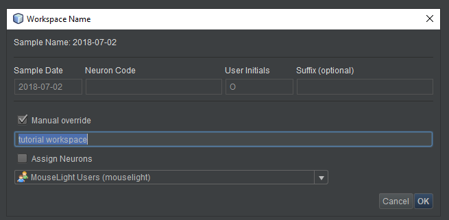
3. By default, the dialog box that pops up provides a template for naming the workspace. For this tutorial, however, click the “Manual override” button to name the workspace without using the template. You can use the default name “new workspace” or enter another name, perhaps “tutorial workspace”. For this tutorial, leave “Assign neurons” unchecked.
4. Click “OK”

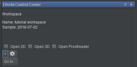
The system will work for a moment, then it will reload the images, this time loading the workspace instead of the sample. You will notice that at the top of the Horta Control Center, the name you gave the workspace will appear just above the sample name now.

In the Data Explorer, this workspace will be located in your “Home” folder (the one with your username next to it in gold), within the “Workspaces” subfolder. You may need to click the refresh button (upper left corner, two arrows in a circle) in the Data Explorer before it shows up.

By default, you are the only person who can see, open, or edit the workspace, save Horta administrators. See the “Basic Operations” section for how to share data.

Adjust colors and save the color model

One immediate advantage of the workspace is the ability to save color settings, which Horta calls the “color model”. Unlike the sample, which is (potentially) shared among many or all users, workspaces often belong to one user. They are therefore appropriate for storing information like color settings, which are often a matter of personal preference.

• First, if the 3D view is not open, click the “Open 3D” checkbox and/or switch to the “Horta 3D” tab as needed.
• Then adjust colors as described in the previous tutorial and shown in screenshots therein. For this sample: set the second purple slider to midway between the left edge and the center lock icons; set the first green slider a bit to the left of the second slider; and hide the third blue channel.
• Next, to save the color model, locate the gear menu in the 3D “Color Sliders” panel, to the right, just under the three channels’ color swatches. Note that the “Horta 2D” tab has its own color sliders. Be sure to use the 3D sliders for this tutorial.
• From the gear menu, choose “Save Color Model to Workspace”.

When you save a color model, all of the color slider settings are saved: channel colors, channel visibility, all sliders, and all locks. From this point forward, when you open this workspace, the color model will be loaded. If you change the color settings later and want to keep them, you’ll need to save them again, however. The color model does not automatically save itself when changed.

The same applies to 2D; you can save the 2D color model (separately) from the gear menu in the 2D color slider area in the Horta 2D tab.

Create a neuron

Now, deep in the third tutorial, we are finally ready to trace a neuron!

In Horta, tracing neurons is done by placing a series of connected point annotations along the neuron signal in the images. These points form one or more trees of points, with each point having one parent point and zero, one, or more child points.

The Horta Control Center contains, below the “Workspace” area, a list of neurons and controls for interacting with neurons.

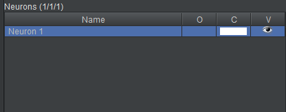
To create a neuron, click the “+” button below the neuron list, just below the “Spatial filter” label. The default name is “Neuron 1”, where the number will be incremented to be larger than existing neurons. You may also give the neuron any name you like, with some restrictions (ie, the * and ? characters can’t be used). You can rename the neuron at any time by right-clicking its name in the neuron list and choosing “Rename”. Once the neuron is created, the name will appear in the neuron list, and the neuron will be selected (highlighted).

The initial color is randomly chosen from a palette of about twenty. If you’d like to change the color of the neuron, click the color swatch to the right of the neuron’s name in the list and choose a new color from the dialog box.

Add points

Let’s find a neuron to trace. You can find any neuron you like (especially if you are not using the 2018-07-02 sample), but we’ll provide the location of a sample neuron if you want to follow along closely. This neuron is chosen for demonstration purposes only! It may not even be traceable along its entire length.

To find the sample neuron:

• Right-click in the 3D view and choose “Reset Horta Rotation” so you are oriented in the default direction
• Click the “Go to…” button in the Horta Control Center (described in more detail in the previous tutorial)
• Enter the following coordinates and click OK: [74130,18910,35035]
  • Remember, if you copy and paste these coordinates, you’ll need to choose the middle icon on the AppStream toolbar and choose “Past to remote session” to transfer the coordinates from your local computer’s clipboard to the AppStream clipboard; once it’s there, you can use control-V to paste as usual
  • See “AppStream Basics” for more information on copying and pasting to and from AppStream

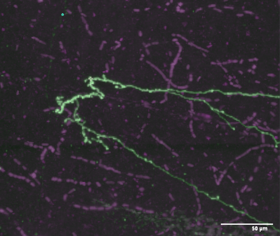
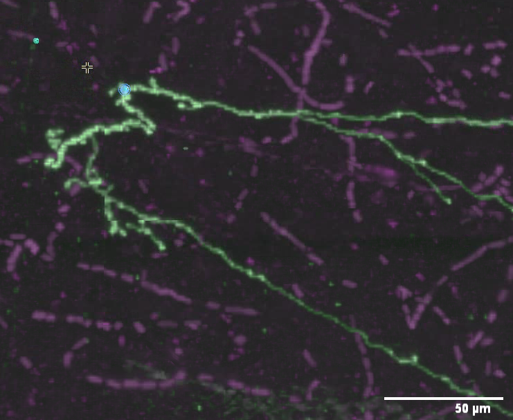
We’re going to trace a small part of the bright neuron making a hairpin turn from the right edge of the screen.

The neuron you want to trace (“Neuron 1” in our case) should be highlighted in the neuron list. If it isn’t, single click it. The list of annotations below the neuron list should be empty at this time, if you’re following the tutorial exactly.

Navigate to the place you want to start tracing. Often this will be the soma of the neuron, but it can be anywhere. For this tutorial, we’ll start placing points in the middle of it. By single-clicking to recenter, dragging the image, and zooming in and out, center the neuron in the view. Feel free to rotate if you like, but to make this tutorial easy to follow from the screenshots, we’ll keep the default rotation.

Now move the mouse pointer over the signal, and over places near the signal but not on it. You’ll notice that a blob with the letter “P” in it appears and reappears as you move the mouse. In fact, you will see that it snaps to the brightest pixels in a small neighborhood around the mouse pointer. If there are no bright pixels, it may not appear at all. This “P” cursor indicates where the point will be placed. Zoom in as much as you need to place the point accurately. Shift-left-click to place the first point when the “P” blob is visible and on top of signal. Near the (x, y, z) location shown above is a good place to place the first point.

The first point appears! It’ll be drawn in the color of the neuron, and it will also have a “P” indicator drawn on it (although that indicator may be difficult to read depending on the strength of the signal nearby). At this point, if you were to rotate the view, you’ll see that the point lies properly on top of the signal in all dimensions. This is another feature of the “P” blob cursor: it senses the correct depth at which to place points. That is, it not only finds bright pixels in the plane of the display, it also finds the brightest pixel along the axis perpendicular to the screen (with a larger search neighborhood).

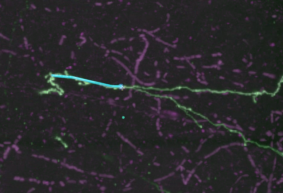
Move the mouse cursor along the neuron signal and shift-click again, working to the right of the screen on the upper segment. Repeat a few times until you have a short string of annotations, points connected by lines. The most recent point you’ve placed always has a (sometimes faint) “P” icon. “P” stands for “Parent”: that is the point to which your next point will be connected.

How densely should you place points? That depends on your intended scientific analysis. If you intend to determine region-to-region connectivity, you can annotate quite sparsely. However, if you intend to calculate neuron length or analyze neuron morphology, you will want to place points with smaller separation. If you’re using the tracing as ground truth for machine learning purposes, you may want near pixel-perfect tracing. In this case, look at the main documentation for the “automatically traced path” feature, in which you can have the computer trace paths between human placed points.

The annotation list and more navigation

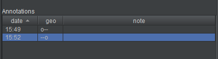
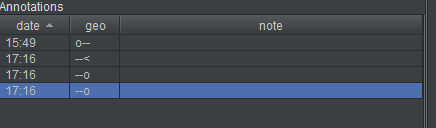
The annotations list now contains a summary of the points you’ve placed. Not every point is listed–that would quickly get unwieldy–but the “interesting” points are. By default, the list includes every root point, endpoint, and branch point. It does not include points along a linear chain. But it also includes points that have some kind of user annotation attached to them (discussed elsewhere in the documentation). If you’re following closely, there will only be two points in the annotation list at this time, the root point and the endpoint.

Both the annotation list and the neuron list can be used for navigation.

• if you double-click a neuron in the neuron list, the view will center on the first point (the root point) in the neuron
• if you double-click on an annotation in the annotation list, the view will center on it

Moving and deleting points

If you make any errors when adding points, there are easy ways to correct them.

If you need to move a point a short distance, left-click and drag it.

• in 2D, you can only drag in the same plane
• in 3D, you can again only drag in the plane of the view; the point does not snap to bright pixels when you drag, so you’ll probably have to rotate and drag multiple times from different angles to fine-tune the location

To delete a point:

• in 2D: left click on it, then press the delete key on the keyboard
• in 2D: right-click on it, then choose “Delete link” from the menu
• in 3D: right-click on it, then choose “Delete Vertex” from the menu

If you delete an annotation in a linear chain, it’ll connect the two surrounding points. You can’t delete the root of the tree or branch points (see below for more on branching). If you need to delete multiple points, see the “Delete subtree” feature described in the “Basic Operations” section.

Branching

You will see that each time you shift-click, the “P” indicator moves to the point you’ve most recently placed. “P” stands for “Parent”: that is the point to which your next point will be connected. This is how you’ll create branches.

If you’ve been following this tutorial closely, your neuron should be approaching a place where the signal branches. Continue adding points headed left until you reach the branch, and place a point directly on the branch location. If you’re tracing on different data, find a convenient branch point, or imagine one (it’s only a tutorial!).

At this point, the next parent icon (“P”) should be on the branch. Choose one arm of the neuron to trace, and add a few points. Now, go back to the branch point and single-click it so it again shows the “P” icon. This indicates that the next point you place will use this point (the branch point) as its parent. Add a few more points along the other branch. You’ve now got a branching structure.

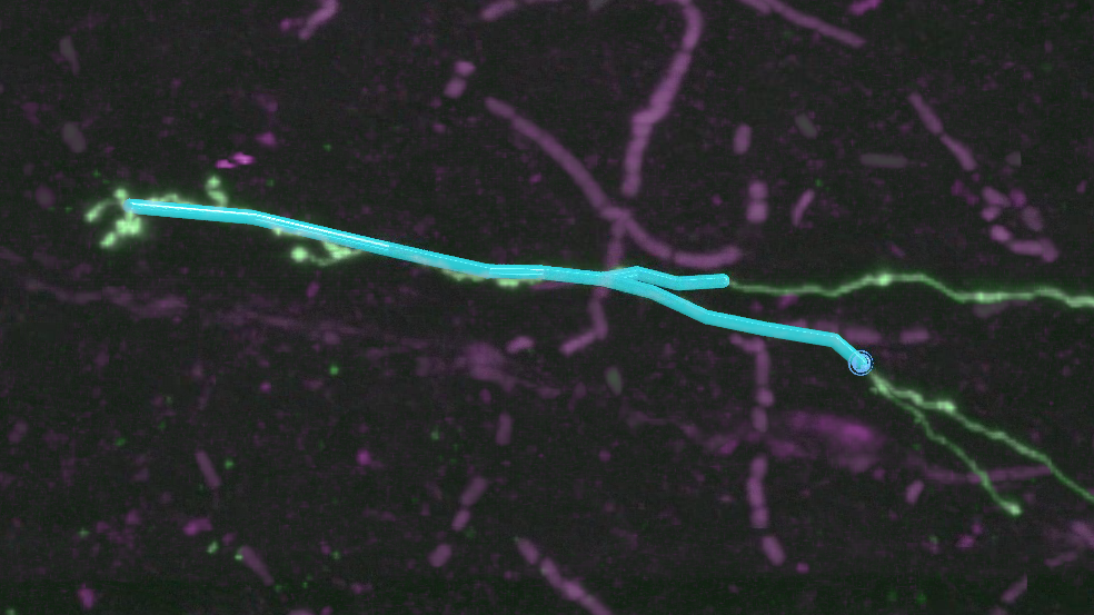
The annotation list now shows the root point, the branch point, and two endpoints.

There are workflows that help you manage the task of tracing a branched structure. See, for example, “Simple workflow with notes and filters” in the “Features” section

Continuing work in the workspace

Annotations are saved to the database immediately after they are placed. This goes for all operations; the application is in constant communication with the database, and all changes are saved immediately. You can quit at any time, and no work will be lost. In this respect, HortaCloud acts more like a mobile application than a desktop application.

When you want to continue work, simple open the workspace from the Data Explorer just as you earlier opened a sample. That is, right-click it in the Data Explorer and choose “Open in Horta”. The neuron data will load immediately. After that, you can choose “Open 3D” and continue work tracing.