This is the multi-page printable view of this section. Click here to print.
HortaCloud Documentation
- 1: Overview
- 2: User manual
- 2.1: Concepts
- 2.2: AppStream Basics
- 2.3: Tutorials
- 2.3.1: Logging in
- 2.3.2: Viewing images
- 2.3.3: Tracing neurons
- 2.3.4: Exporting and importing neurons
- 2.4: Basic Operations
- 2.5: Features
- 2.6: Reference
- 2.7: Synchronized Folders
- 2.8: Reporting issues
- 3: Administration guide
- 3.1: AWS
- 3.1.1: Estimated Costs
- 3.1.2: Best Practices
- 3.1.3: Deployment Steps
- 3.1.4: Backup & Restore
- 3.1.5: Upgrading
- 3.1.6: Data Import
- 3.1.7: Troubleshooting
- 3.2: Bare metal
- 3.2.1: Two-server deployment
- 3.2.2: Three-server deployment
- 3.2.3: Installing Docker
- 3.2.4: Deploying JACS
- 3.2.5: Deploying ELK
- 3.2.6: Self-signed Certificates
- 3.2.7: Storage volumes
- 3.2.8: Data import
- 3.2.9: Troubleshooting
- 4: Developer's guide
- 4.1: Getting started
- 4.2: Single server deployment
- 4.3: System Overview
- 4.3.1: Persistence
- 4.3.2: Tiled Imagery
- 4.3.3: Event Handling/Communication
- 4.4: Contribution guidelines
- 5: Support
- 6: Editing the documentation
1 - Overview
HortaCloud is a streaming 3D annotation platform for large microscopy data that runs entirely in the cloud. It is a free, open source research software tool, developed by Janelia Research Campus.
It combines state-of-the-art volumetric visualization, advanced features for 3D neuronal annotation, and real-time multi-user collaboration with a set of enterprise-grade backend microservices for moving and processing large amounts of data rapidly and securely. HortaCloud takes advantage of cloud-based Virtual Desktop Infrastructure (VDI) to perform all 3D rendering in cloud-leased GPUs which are data-adjacent, and only transfer a high-fidelity interactive video stream to each annotator’s local compute platform through a web browser.
What is it good for?: HortaCloud is a powerful tool for 3D visualization and annotation of large-scale microscopy data. It has been used to trace axons across the entire mouse brain by Janelia’s MouseLight Team Project.
What is it not good for?: HortaCloud is a very specialized tool for sparse microscopy data. It is not intended for annotation of dense data sets, such as electron microscopy (EM) imagery.
What makes HortaCloud unique?: Leveraging state-of-the-art services on AWS allows HortaCloud to run entirely in the cloud, making it possible to visualize terabyte-scale 3D volumes without moving all of that data over the Internet (see diagram below).

Where should I go next?
If you are a HortaCloud user, read through the User Manual to get familiar with the tools.
If you are a system administrator or developer looking to deploy an instance of HortaCloud, start with the AWS Deployment Guide.
2 - User manual
The sections below describe Horta’s basic and advanced features. Generally the sections listed below should be read in the order listed.
Note on Horta versions
The Horta application exists in two versions that come from a common code base. The cloud version (HortaCloud) that is available here is a reduced version of the desktop version (Janelia Workstation). In fact, we’ll often use the word “workstation” to refer to the Horta application in either form.
When there are differences between the two versions, they will be noted with “(HortaCloud)” and “(desktop)”. If the differences are more substantial, they will be presented like this:
HortaCloud only
In HortaCloud, the following control behaves differently from the desktop version.Desktop only
The following features is only available in the desktop version of the Janelia Workstation.The major user-visible differences between the two versions are:
- HortaCloud does not have access to the local file system or clipboard and requires additional steps to import or export data via those routes (see AppStream Basics section for details)
- HortaCloud datasets typically only include low-resolution 2D data, so some 2D tools are not as useful or may not function in the absence of high-resolution data (eg, automatic path tracing)
- the desktop Janelia Workstation contains tools for viewing, annotating, and managing other unrelated Janelia datasets
2.1 - Concepts
Data
Light microscopes of various kinds can now image an entire fly or mouse brain (eg, resonant scanning two photon with integrated vibrotome or Bessel light sheet). Horta is capable of displaying and annotating the resulting multi-terabyte datasets. The details of how the data should be prepared for use in Horta is covered in the Horta Reference section. In general, though, the data will have these properties:
- size: generally limited by disk space (local or cloud)
- channels: two channels are supported and tested; three channels are supported but not well tested; four or more channels are possible but would require more development
- location: the data will be on a storage system accessible to the image server
- (HortaCloud) AWS S3 bucket
- (desktop) local or networked storage available to the workstation servers
- the file path to the data should be known to the user if they will be creating samples manually
- arrangement: the 2D and 3D images are arranged in multi-resolution octrees; details are covered in the reference section, but the user doesn’t need to know them
Software & tasks
Horta includes the Horta 2D viewer, which is the 2D, plane-by-plane, viewing and annotation tool, and the Horta 3D viewer, which supports viewing and annotating the data in three dimensions. The two viewers connect to common data editing and storage functions, many of which can be viewed in the Horta Control Center.
Horta is designed for a variety of tasks:
- viewing data: panning, zooming in and out, and scrolling through planes; brightness and contrast adjustment
- skeletal tracing of neurons: tracer places connected points on the signal
- text annotation: each point can have arbitrary text added to it
- import/export: skeletons can be imported or exported as SWC files; text notes are imported/exported as JSON (see reference section for details)
Why the name 'Horta'?
“Horta” is the name of a tunneling silicon based lifeform from the Star Trek original series episode 25 “The Devil in the Dark”. Neuron traces in 3D resemble the tunnels such a creature might make in the ground. “Horta” can also be conveniently backronymed as “How Outstanding Researchers Trace Axons”.Workflows
The basic tools can be used to implement a variety of workflows. For example, a user may trace a neuron entirely on their own. Or two users may trace the same neuron, export their results, and a later user may compare those results either by importing them both back in to the workstation or using other tools. If computational methods can trace neurons and export the results as SWC files, those results can be imported into the workstation for validation and/or correction and extension by later users. This flexibility supports neuron reconstruction at both small and large scales.
Jargon
- basic objects in Horta:
sample: the data; specifically, the object in the workstation that represents a particular image dataset; it’s independent of user, and it’s all you need if you are only viewing the dataworkspace: the object in the workstation that collects a set of annotations (traced neurons and text annotations); it is owned by a user or group, and it contains neuronsneuron: the object that holds the traced neuron skeletons; a neuron usually contains one or more neuritesneurite: a single skeleton or tree; a group of annotations with parent-child relationships, all tracing back to a single root without a parentannotation: a single point that may have zero or one parent and zero or more children; annotations are sometimes called anchorstag: a word or phrase attached to a neuron; it may be used in filtering the neuron list or in controlling neuron appearanceowner: a username or group that owns the neuron; if a neuron is owned by a user, only they may change it; if a neuron is owned by a group, any member of the group may take sole ownership of the neuron (and then change it)
- data and data formats:
tilesoroctree: the files holding the 2D dataktx tiles: the files holding the 3D dataSWC file: a common multi-column text file format for storing neuron skeletonsJSON file: a common structured text file format used to import/export text annotations
- tracing methods & workflows:
manual: a tracer clicks along the signal in the data to create a neuron skeletonsemi-automated: a computer program partially traces the signal in a dataset; the fragments are imported into the workstation; a tracer connects and/or extends fragments as needed to produce the skeleton
2.2 - AppStream Basics
The AppStream environment
In general, the AppStream environment behaves like a Windows desktop computer running a single application, Horta. Because it’s running in a browser, though, there are some important differences. Many of them are managed via the AppStream toolbar at the top of the screen.
Older AppStream toolbar:

Newer AppStream toolbar:

Data import and export: file system, cloud storage, and clipboard
Note: The AppStream toolbar may differ slightly; the icon positions referred to below are for the older AppStream version.
Web browsers are constrained with respect to how they read and write data on a computer, and applications running in virtual machines displayed in a browser, even more so.
File system access: The third icon from the left opens a dialog showing “My Files”, and within it, a “Temporary Files” location. This is a file location on the remote computer running Horta and Horta can read and write to. You can then transfer files from that location to your local computer via the “My Files” dialog box. See “Importing Data” and “Exporting Data” in the “Basic Operations” section for more details.
Cloud storage: Files can also be transferred to cloud storage. The exact services available will depend on your local deployment. To connect to a cloud storage provider, click the “My Files” icon on the tool boar, then click the “Add Storage” button to connect to an available synchronized folder. Contact your local administrator for details on what cloud storage is available in your instance.
Clipboard access: If you copy anything in Horta to the clipboard, it’s only accessible on the remote computer. The fourth icon from left on the toolbar will transfer the remote clipboard’s contents to the local clipboard.
Windows and screens
Horta users often want to see the 2D and 3D views simultaneously, or they want a maximum 3D view while leaving room for the Data Explorer and/or Horta Control Center. To enable use of multiple monitors, click the seventh icon from left on the toolbar. There is also a full-screen mode enabled via the sixth icon.
The second icon on the toolbar shows all windows, in case you undock a Horta Window and then lose it behind a larger window. There’s also a terminal window from which Horta is initially run; this can be ignored. If you close it, it will close Horta.
Quitting and relaunching Horta
Sometimes Horta does have issues. Often reloading data by reopening a workspace will clear them up. If not, to relaunch the application again without ending the AppStream session, choose File > Exit or click the “x” at top right. Then relaunch the application by clicking the first icon in the toolbar and choosing “Horta Workstation” again.
Ending the session
Generally sessions will automatically close after a period of inactivity. To end the session manually, you can choose “End Session” from the drop-down menu on the top-right toolbar button.
Remember that when you end a session, some data that is stored on the remote computer will be lost:
Volatile data:
- files in “MyFiles/Temporary Files”
- information on the clipboard
All other data (sample data, workspace data, annotations, notes, etc.) is stored in the database and is not lost when a session ends.
Any data you wish to preserve (e.g., exported neuron SWC files) should be moved from “My Files” to either local storage or cloud storage before you end the session.
Reconnecting
If your browser window is accidentally closed, your session is not lost. Simply repeat the login steps, and you will be reconnected to the session, even if from a different browser and/or computer.
2.3 - Tutorials
Each of the tutorials builds on the preceding tutorials, and they should be completed in order.
2.3.1 - Logging in
In this tutorial, we’ll go over the steps needed to log into HortaCloud and start the Horta application.
HortaCloud only
This tutorial applies to HortaCloud only.Prerequisites
- You should know the URL for the HortaCloud instance that you will be using.
- The administrator of the instance should have created an account for you.
- You should know the username and password for that account.
The screenshots below were taken from the Janelia instance in June 2022.
Steps
The steps to log in to HortaCloud and starting the Horta application are similar to the steps for many web applications. The procedure is straightforward, but we’ve provided screenshots of every step to help troubleshooting when things go wrong.
Navigate to your HortaCloud website’s URL in your browser.
You are probably already on the site, if you’re reading this documentation! Click the button on the right labeled “Login to HortaCloud”.
All major browsers are supported: Safari, Google Chrome, Mozilla Firefox, and Microsoft Edge.

Enter your username and password given to you by your local administrator in the entry fields, then click the “Login” button.
On this page, there are also links for changing your password and for requesting a password reset if you have forgotten your password.

Click “AppStream Login” to continue.
This screen also contains a change password link, and if you are a Horta application administrator, you will also see tools for managing users and groups in Horta.

Click “Horta Workstation” to start the application.
This is currently the only application in HortaCloud.

Wait for application startup
As the application starts, which can take a couple minutes, you will see a wait screen (first image below). The percentage should steadily increase. After that, you will see a brief console screen (second image below), then the Horta application itself (third image below).
The list of folders you see in the “Data Explorer” in Horta will be different and will depend on what data is available in your instance and which data you personally have permissions to see.


Troubleshooting
In most cases, if you have trouble launching the Horta application, you should contact your local HortaCloud administrator. If the application launches but you do not see the expected data, you should contact the local Horta application administrator. Of course, these may be the same person.
Ending your session
You can end your session by clicking on the rightmost icon on the AppStream toolbar and choosing “End Session”.

2.3.2 - Viewing images
In this tutorial, we’ll go over the steps needed to load images in Horta and view them.
HortaCloud-focused
This tutorial is focused on HortaCloud. However, most of it applies to the desktop version of Horta as well. If you can launch Horta on the desktop, and you see data in the Data Explorer, you should be able to follow most of the other steps of the tutorial.Prerequisites
- You should be able to log into HortaCloud and launch the Horta application, as detailed in the previous tutorial.
- Your HortaCloud instance should have access to the Janelia MouseLight data on Amazon AWS S3.
- If not, you should have access to some similar data in your HortaCloud instance.
Steps
Start the Horta Application
Launch the Horta application. See the previous tutorial “Logging in” for more detail.
Locate and examine data in the Data Explorer
The “Data Explorer”, which appears by default in the upper left panel of Horta, shows a representation of all the data in Horta that you are allowed to see. This data is organized in folders, both created by the system and created by users. The exact list of folder you see will differ depending on which data you have permission to see.
Click on the triangle to the left of the folder named Home with the owner mouselight, which appears immediately to the right of the folder name, in yellow. This will open the folder to show its contents.
Click on the triangle to the left of the “3D Tile Microscope Samples” folder, also owned by mouselight. You will see a long list of samples, indicated by a green flask icon. Each of these sample represents a group of image files on disk or in an AWS S3 bucket.
For this tutorial, we’re going to look at one of the Janelia Mouse Light samples, the 2018-07-02 sample. Scroll down the list of samples until you see it. Left-click on the sample to select it. You will see information appear in the “Data Inspector”, located just below the Data Explorer.
The three tabs of the Data Inspector each show information about the sample. The “Attributes” tab contains typical metadata like name, creation/modification date, and globally unique identifier (GUID). It also shows the sample’s owner and the location of the image files that belong to the sample. The “Permissions” tab shows which users or groups can read or write to the data. There’s also a button which allows someone to grant permissions to other users to see or edit the data. The third tab, “Annotations”, is not used by Horta and is only used with other tools in the desktop workstation client.

Open a sample in Horta
Now that we’ve located the 2018-07-02 sample, it’s time to open it in Horta.
Do one of two things:
- Right-click the sample, and choose “Open in Horta”.
- Left-click the sample to select it; then choose
Horta>Open in Hortafrom theActionsmenu.
At this point, not a lot will visibly happen. When you open a sample in Horta, all that happens is that the dataset’s metadata is loaded into the application. The images themselves are not yet loaded. You will see that in the “Horta Control Center” panel at right, near the top below the “WORKSPACE” heading, the “Sample” field will now show the name “2018-07-02”. That’s all (screenshot below). In the next tutorial (“Tracing neurons”), we’ll see that opening a workspace in Horta populates much more information in the UI. The “Concepts” section of the documentation has more information on the difference between samples and workspaces.

Open the Horta 3D window
It’s time to finally look at some images. For this demonstration, we’ll start with the 3D images. Near the top of the Horta Control Center, under the “VIEWS” heading, find the checkbox labeled “Open 3D”. Click it so it’s checked.
You will see a window tab titled “Horta 3D” open in the center panel. The first 3D images will also load. Initially, it’ll be underwhelming. Probably you’ll see one small bright rectangle in the center of the screen. In the next section, we’ll see how to adjust the color. For now, if you left-click in the 3D window, more data will load to cover most of the window.


Explore the data in 3D
Adjust colors
The default color settings are not good; in general, the data will appear to be a washed out bright, light blue/purple. In order to adjust the color, first we need to go to the “Windows” menu and choose Horta > Color Sliders.
Often when the sliders are first opened, their panel will not be the correct height. You can adjust this. Like other panels in Horta, the color slider panel may be resized and docked or undocked from the main window as you like.
Also, when the color sliders are first opened, often the 3D image will be redrawn, or potentially not drawn at all. If this occurs, left-click in the 3D window to trigger a redraw.
Even though the data only has two channels (a signal channel and a reference channel), you’ll see three sliders. The third blue slider has a specialized use that we’re not going to cover in this tutorial. Click the eye next to the blue slider, and the blue channel will be hidden.
In practice, you will likely spend a lot of time tuning the color settings so the desired biological structures are most visible. For this tutorial, we’ll cover a few simple steps to make the data more visible:
- First, you can optionally display the numeric values of the sliders by clicking the
#button at the far right of each color slider, just before the color swatch. This is useful if you want to adjust values finely. It’s also useful to communicate the values to another user. But note if you want to import or export all of the color settings at once, you can do so using those options on the gear menu in the lower right corner of the color slider panel. - Click the eye icon to the left of the top, green slider. This turns the green channel data invisible.
- Now drag the leftmost slider of the middle, purple slider to the right. Do this until the blocky, purple background of the image tiles disappears and you can see the purple outline of the brain. For this data, you’ll be dragging the slider until it’s midway between the left edge and the center lock icon below the sliders. If you have the numbers showing, set “Min” to around 15600.
- Now do it again for green. Click the eye next to the green slider to show the green channel, and the eye next to the purple channel to hide it. Drag the leftmost slide of the green bar until, again, the blocky background disappears and the brain outline is visible. For this data, try setting it a bit to the left of the left purple slider. That’s around a value of 12200 for “Min”.
- Click the eye next to the purple slide so both data channels are visible again.
At this point (screenshot below), the labeled neurons, though, stand out in green against the purple background. Feel free to experiment with the other sliders. It’s a matter of personal preference. Some tracers prefer to adjust the settings until the background is nearly invisible, so that the neuron signal is prominent, even if dim.
Note: Color settings are not saved for samples! In the next tutorial, we’ll see how these settings are saved in workspaces.

Pan, zoom, rotate
Navigating the 3D data is done using the mouse.
To navigate in space (pan):
- left-click to center on a location
- left-drag to move the image in the view plane
- as you navigate, images will be loaded and unloaded
To zoom in and out:
- use the scroll wheel to zoom in or out; as you zoom, higher or lower resolutions images will be loaded
- note that as you zoom in, you will see less and less of the thickness of the brain; that is, the displayed data will come from a projection depth that is smaller, allowing you to more clearly isolate smaller structures as you zoom in
To rotate in 3D:
- middle-click and drag, or hold down the shift key and left-click and drag; the cursor will change to two curved arrows, and the image will rotate in three dimensions

Open the Horta 2D window
HortaCloud
Note that HortaCloud does not store high-resolution 2D images! When you zoom in, the images will be blurry.
In the Horta desktop application, when you zoom in, higher-resolution images will automatically be loaded.
Loading the 2D images is done just like for 3D. Near the top of the Horta Control Center, in the “VIEWS” section, find the checkbox labeled “Open 2D”. Click it so it’s checked.
You will see a window tab titled “Horta 2D” open in the center panel. The first 2D images will also load.

Explore the data in 2D
Adjust colors
As with 3D, the default color settings are almost never useful, and we’ll quickly adjust them to make the data more visible. In practice, you will likely spend a lot of time tuning the color settings so the desired biological structures are most visible.
The colors of the two data channels are controlled by the sliders and buttons at the bottom of the middle panel in the “Horta 2D” tab. They are distinct from the sliders used to adjust the 3D colors.
NOTE: Sometimes the color slider do not draw correctly when the sample initially opens in 2D. If this is the case, you will see two small checkboxes and two small plus signs at the right of the empty area below the 2D image. Toggle either on of the check boxes off and on, and the sliders should redraw.
Here are the steps to make some minimal adjustments to the colors:
- As before, you can optionally display the numeric values of the sliders by clicking the
#button at the far right of each color slider - Click the eye icon to the left of the top, green slider. This turns the green channel data invisible.
- Now drag the leftmost slider of the lower, purple slider to the right. Do this until the blocky, purple background of the image tiles disappears and you can see the purple outline of the brain. For this data, you’ll be dragging the slider until it’s midway between the left edge and the center lock icon below the sliders. Try a value of “Min” = 15200.
- Now do it again for green. Click the eye next to the green slider to show the green channel, and the eye next to the purple channel to hide it. Drag the leftmost slide of the green bar until, again, the blocky background disappears and the brain outline is visible. For this data, try a location just to the left of the middle purple slider. Try “Min” = 11800.
- Click the eye next to the purple slide so both data channels are visible again.
At this point (screenshot), the labeled neurons stand out in green against the purple background. Feel free to experiment with the other sliders. Again, it’s a matter of preference, your data, and your display, among other things.

Note: Color settings are not saved for samples! In the next tutorial, we’ll see how these settings are saved in workspaces.
Pan, scroll through z, zoom
Navigating the 2D data is done using the mouse.
To navigate in the x-y plane, you can:
- double-left-click on any location to center the view on that point
- middle-click and drag to pan the image to any location
To navigate along the z-axis, you can:
- use the scroll wheel to change the visible plane
- drag the horizontal slider below the 2D view to change the visible plane
- change the plane number visible in the plane number box to the right of the plane slider by either typing a plane number in the box, or by clicking the up and down arrows in the box
To zoom the image:
- hold down the shift key and spin the scroll wheel
- drag the vertical slider to the right of the 2D view
- remember, HortaCloud does not has high-resolution 2D images; when you zoom in, it will be blurry!
x, y, z locations
Status bars
As you move the mouse cursor in either the 2D or 3D windows, you will see the x, y, z location of the cursor displayed in the status bars.
- in 3D, the status bar is at the very bottom of the Horta application window
- in 2D, the status bar is at the bottom of the 2D window; the 3D status bar in this case is not accurate, and it does not update
- in both cases, the
x, y, zlocation is given in microns (µm), as a floating-point number
The screenshot below shows both status bars, with the 3D bar at the bottom and the 2D bar above it.

Copying location values
You can copy the the current x, y, z location to the clipboard by right-clicking in the view.
- in 3D, right-click and choose “Copy Micron Location to Clipboard”
- in 2D, right-click and choose “Copy Micron Coords to Clipboard”
- in both cases, the copied text has the following form:
[68665.88,48154.89,26670.117]- this is convenient for pasting into eg Matlab or Python
- (HortaCloud) see the “AppStream Basics” section in this documentation for how to transfer the data from AppStream’s clipboard to your local system’s clipboard
Go to point
If you know the x, y, z location you’d like to navigate to, and that data is on the clipboard, click the “Go to location…” button that appears in the “VIEWS” section in the Horta Control Center. Paste in the data from the clipboard and click “OK”. Both the 2D and 3D views will navigate to put that point at the center of the view without changing the zoom level.
Details:
- the values should be in microns
- you can paste in
x, y, zcoordinates or justx, y; in the latter case, the currentzvalue will not change - any brackets or commas will be removed
- thus you can copy and paste from Horta, or from eg Matlab or Python
Again, HortaCloud users should see “AppStream Basics” for how to move data from your local system to the AppStream Clipboard.
2.3.3 - Tracing neurons
In this tutorial, we’ll go over the steps needed to begin tracing a neuron in Horta in the 3D view.
HortaCloud-focused
This tutorial is focused on HortaCloud. However, most of it applies to the desktop version of Horta as well. If you can launch Horta on the desktop, and you see data in the Data Explorer, you should be able to follow most of the other steps of the tutorial.3D-focused
This tutorial doesn’t cover tracing in 2D in detail. Most of it is the same (creating workspaces, neurons, shift-click to add points), but there are some slight differences. See the “Basic Operations” section for details on 2D tracing.
For HortaCloud, 2D tracing is rarely useful, as HortaCloud does not usually contain high-resolution 2D data. You’re not going to be able to accurately place annotations with the low-resolution data.
Prerequisites
- You should be able to log into HortaCloud and launch the Horta application, as detailed in the first tutorial.
- You should be able to open a sample in 3D and navigate the data, as detailed in the second tutorial.
- Your HortaCloud instance should have access to the Janelia MouseLight data on Amazon AWS S3.
- If not, you should have access to some similar data in your HortaCloud instance.
Steps
Start the Horta Application and open a sample in Horta
As detailed in the previous two tutorials:
- Launch HortaCloud
- Locate the
2018-07-02sample in the Data Explorer and open it in the Horta Control Center - Open the sample in the 3D viewer
Create a workspace
The sample that is listed in the Data Explorer, that we’ve opened in Horta, is the representation of the image data in the database. In general, a user never needs to change this information–it’s a static snapshot of the image data. The sample is shared among all users who will work with that dataset.
A workspace, by contrast, contains the neurons that a user has traced. The workspace initially belongs to and can only be seen by the user that created it, but it can then be shared with other users and/or groups.
To create a workspace:
- Open a sample in Horta (as done in the previous step); this is the dataset that the neuron tracing will be associated with
- In the Horta Control Center at right, in the “WORKSPACE” section, click the button labeled “New workspace…”.
- By default, the dialog box that pops up provides a template for naming the workspace. For this tutorial, however, click the “Manual override” button to name the workspace without using the template. You can use the default name “new workspace” or enter another name, perhaps “tutorial workspace”. For this tutorial, leave “Assign neurons” unchecked.
- Click “OK”

The system will work for a moment, then it will reload the images, this time loading the workspace instead of the sample. You will notice that in the “WORKSPACE” section of the Horta Control Center, the name you gave the workspace will appear just above the sample name now.

In the Data Explorer, this workspace will be located in your “Home” folder (the one with your username next to it in gold), within the “Workspaces” subfolder. You may need to click the refresh button (upper left corner, two arrows in a circle) in the Data Explorer before it shows up.
By default, you are the only person who can see, open, or edit the workspace, save Horta administrators. See the “Basic Operations” section for how to share data.
Adjust colors and save the color model
One immediate advantage of the workspace is the ability to save color settings, which Horta calls the “color model”. Unlike the sample, which is (potentially) shared among many or all users, workspaces often belong to one user. They are therefore appropriate for storing information like color settings, which are often a matter of personal preference.
- First, if the 3D view is not open, click the “Open 3D” checkbox and/or switch to the “Horta 3D” tab as needed.
- Then adjust colors as described in the previous tutorial and shown in screenshots therein. For this sample: set the second purple slider to midway between the left edge and the center lock icons; set the first green slider a bit to the left of the second slider; and hide the third blue channel.
- Next, to save the color model, locate the gear menu in the 3D “Color Sliders” panel, to the right, just under the three channels’ color swatches. Note that the “Horta 2D” tab has its own color sliders. Be sure to use the 3D sliders for this tutorial.
- From the gear menu, choose “Save Color Model to Workspace”.
When you save a color model, all of the color slider settings are saved: channel colors, channel visibility, all sliders, and all locks. From this point forward, when you open this workspace, the color model will be loaded. If you change the color settings later and want to keep them, you’ll need to save them again, however. The color model does not automatically save itself when changed.
The same applies to 2D; you can save the 2D color model (separately) from the gear menu in the 2D color slider area in the Horta 2D tab.
Create a neuron
Now, deep in the third tutorial, we are finally ready to trace a neuron!
In Horta, tracing neurons is done by placing a series of connected point annotations along the neuron signal in the images. These points form one or more trees of points, with each point having one parent point and zero, one, or more child points.
The Horta Control Center contains, below the “WORKSPACE” and “VIEWS” sections, a “NEURONS” section that contains a list of neurons and controls for interacting with neurons.
To create a neuron, click the “Add…” button below the neuron list. The default name is “Neuron 1”, where the number will be incremented to be larger than existing neurons. You may also give the neuron any name you like, with some restrictions (eg, the * and ? characters can’t be used). You can rename the neuron at any time by right-clicking its name in the neuron list and choosing “Rename”. Once the neuron is created, the name will appear in the neuron list, and the neuron will be selected (highlighted).
The initial color is randomly chosen from a palette of about twenty. If you’d like to change the color of the neuron, click the color swatch to the right of the neuron’s name in the list and choose a new color from the dialog box.

Add points
Let’s find a neuron to trace. You can find any neuron you like (especially if you are not using the 2018-07-02 sample), but we’ll provide the location of a sample neuron if you want to follow along closely. This neuron is chosen for demonstration purposes only! It may not even be traceable along its entire length.
To find the sample neuron:
- Right-click in the 3D view and choose “Reset Horta Rotation” so you are oriented in the default direction
- Click the “Go to location…” button in the “VIEWS” section of the Horta Control Center (described in more detail in the previous tutorial)
- Enter the following coordinates and click OK:
[74130,18910,35035]- Remember, if you copy and paste these coordinates, you’ll need to choose the middle icon on the AppStream toolbar and choose “Past to remote session” to transfer the coordinates from your local computer’s clipboard to the AppStream clipboard; once it’s there, you can use control-V to paste as usual
- See “AppStream Basics” for more information on copying and pasting to and from AppStream
We’re going to trace a small part of the bright neuron making a hairpin turn from the right edge of the screen.

The neuron you want to trace (“Neuron 1” in our case) should be highlighted in the neuron list. If it isn’t, single click it. The list of annotations below the neuron list should be empty at this time, if you’re following the tutorial exactly.
Navigate to the place you want to start tracing. Often this will be the soma of the neuron, but it can be anywhere. For this tutorial, we’ll start placing points in the middle of it. By single-clicking to recenter, dragging the image, and zooming in and out, center the neuron in the view. Feel free to rotate if you like, but to make this tutorial easy to follow from the screenshots, we’ll keep the default rotation.
Now move the mouse pointer over the signal, and over places near the signal but not on it. You’ll notice that a blob with the letter “P” in it appears and reappears as you move the mouse. In fact, you will see that it snaps to the brightest pixels in a small neighborhood around the mouse pointer. If there are no bright pixels, it may not appear at all. This “P” cursor indicates where the point will be placed. Zoom in as much as you need to place the point accurately. Shift-left-click to place the first point when the “P” blob is visible and on top of signal. Near the (x, y, z) location shown above is a good place to place the first point.

The first point appears! It’ll be drawn in the color of the neuron, and it will also have a “P” indicator drawn on it (although that indicator may be difficult to read depending on the strength of the signal nearby). At this point, if you were to rotate the view, you’ll see that the point lies properly on top of the signal in all dimensions. This is another feature of the “P” blob cursor: it senses the correct depth at which to place points. That is, it not only finds bright pixels in the plane of the display, it also finds the brightest pixel along the axis perpendicular to the screen (with a larger search neighborhood).
Move the mouse cursor along the neuron signal and shift-click again, working to the right of the screen on the upper segment. Repeat a few times until you have a short string of annotations, points connected by lines. The most recent point you’ve placed always has a (sometimes faint) “P” icon. “P” stands for “Parent”: that is the point to which your next point will be connected.

How densely should you place points? That depends on your intended scientific analysis. If you intend to determine region-to-region connectivity, you can annotate quite sparsely. However, if you intend to calculate neuron length or analyze neuron morphology, you will want to place points with smaller separation. If you’re using the tracing as ground truth for machine learning purposes, you may want near pixel-perfect tracing. In this case, look at the main documentation for the “automatically traced path” feature, in which you can have the computer trace paths between human placed points.
The annotation list and more navigation
The annotations list, in the “ANNOTATIONS” section, now contains a summary of the points you’ve placed. Not every point is listed–that would quickly get unwieldy–but the “interesting” points are. By default, the list includes every root point, endpoint, and branch point. It does not include points along a linear chain. But it also includes points that have some kind of user annotation attached to them (discussed elsewhere in the documentation). If you’re following closely, there will only be two points in the annotation list at this time, the root point and the endpoint.

Both the annotation list and the neuron list can be used for navigation.
- if you double-click a neuron in the neuron list, the view will center on the first point (the root point) in the neuron
- if you double-click on an annotation in the annotation list, the view will center on it
Moving and deleting points
If you make any errors when adding points, there are easy ways to correct them.
If you need to move a point a short distance, left-click and drag it.
- in 2D, you can only drag in the same plane
- in 3D, you can again only drag in the plane of the view; the point does not snap to bright pixels when you drag, so you’ll probably have to rotate and drag multiple times from different angles to fine-tune the location
To delete a point:
- in 2D: left click on it, then press the delete key on the keyboard
- in 2D: right-click on it, then choose “Delete link” from the menu
- in 3D: right-click on it, then choose “Delete Vertex” from the menu
If you delete an annotation in a linear chain, it’ll connect the two surrounding points. You can’t delete the root of the tree or branch points (see below for more on branching). If you need to delete multiple points, see the “Delete subtree” feature described in the “Basic Operations” section.
Branching
You will see that each time you shift-click, the “P” indicator moves to the point you’ve most recently placed. “P” stands for “Parent”: that is the point to which your next point will be connected. This is how you’ll create branches.
If you’ve been following this tutorial closely, your neuron should be approaching a place where the signal branches. Continue adding points headed left until you reach the branch, and place a point directly on the branch location. If you’re tracing on different data, find a convenient branch point, or imagine one (it’s only a tutorial!).
At this point, the next parent icon (“P”) should be on the branch. Choose one arm of the neuron to trace, and add a few points. Now, go back to the branch point and single-click it so it again shows the “P” icon. This indicates that the next point you place will use this point (the branch point) as its parent. Add a few more points along the other branch. You’ve now got a branching structure.

The annotation list now shows the root point, the branch point, and two endpoints.

There are workflows that help you manage the task of tracing a branched structure. See, for example, “Simple workflow with notes and filters” in the “Features” section
Continuing work in the workspace
Annotations are saved to the database immediately after they are placed. This goes for all operations; the application is in constant communication with the database, and all changes are saved immediately. You can quit at any time, and no work will be lost. In this respect, HortaCloud acts more like a mobile application than a desktop application.
When you want to continue work, simple open the workspace from the Data Explorer just as you earlier opened a sample. That is, right-click it in the Data Explorer and choose “Open in Horta”. The neuron data will load immediately. After that, you can choose “Open 3D” and continue work tracing.
2.3.4 - Exporting and importing neurons
In this tutorial, we’ll go over how to export and import traced neurons from/to Horta.
Prerequisites
- You should be able to log into HortaCloud and launch the Horta application, as detailed in the first tutorial.
- You should be able to open a workspace in 3D and navigate the data, as detailed in the second tutorial.
- You should be able to create and add points to a neuron, as detailed in the third tutorial.
Steps
Open the workspace
Launch HortaCloud and open the workspace created in the previous tutorial, or any other workspace that you can trace in.
Exporting neurons as SWC files
Once you’ve finished tracing a neuron, you will probably want to export the data for analysis or visualization in another piece of software. Horta supports import and export to the standard SWC file format. Details of the SWC format can be found in the “Reference” section.
To export a traced neuron:
- Right click on its name in the neuron list and choose “Export SWC File”. A file dialog box will open.
- Name the file whatever you like. An extension of “.swc” is strongly recommended. The two options on the right are discussed in the “Basic Operations” section. The defaults are appropriate almost all of the time.
- Choose the export location. For desktop, choose any location you like on your hard drive. For HortaCloud, we need to save to an intermediate location first. At the top of the dialog box, click the “Save in” drop-down menu and choose “Temporary Files”.

- Click “OK”. A “Background Tasks” window will open with a progress bar. This operation is very fast, and you may not even see the bar before it’s filled. For desktop Horta, you’re done after this step.
- For HortaCloud users, you now need to download your file(s) from the “Temporary Files” location on AppStream. The AppStream toolbar appears at the top of the browser’s content window, above the top of the Horta main window. Click the third icon from left, which has a tooltip of “My Files”.
- In the new dialog box that opens, click “Temporary Files”. This is a web view into the folder where you exported your neuron. At the right end of the row for each file in this directory is a downward facing chevron. Click it and choose “Download” from the drop-down menu. Depending on your browser, you may be prompted to choose a location, or the file may be downloaded to your default downloads location. Also depending on your browser, you may need to authorize or confirm the download from the AppStream site.

Temporary means temporary!
The name “Temporary Files” is accurate! The files in this location will be deleted when your session ends. You must download any exported neurons to your local computer in the same session in which you exported them.Importing neurons from SWC files
Importing neurons from SWC files is basically the same as exporting, in reverse. Again, the HortaCloud procedure involves an intermediate location.
If you’ve been using the Janelia 2021-03-17 sample for your test, you can download a test neuron to import (right-click and download the linked file). If you don’t have access to the Janelia sample we’re using in these tutorials, you can test importing a neuron into your own sample and workspace by simply exporting any neuron (as in the previous section), deleting the neuron using the “-” button under the neuron list, and then reimporting the same neuron.
To import a traced neuron:
- Open a workspace that corresponds to the same sample the neuron was exported from. In other words, the exported neuron’s SWC file must be using the same coordinate system and same scale as the target sample. If not, the imported neuron will not lie on top of the neuron signal in the images. In many cases, it will be imported somewhere in space far from the brain imagery.
- (HortaCloud only) Upload the SWC file to AppStream. Click the “My Files” icon on the AppStream toolbar (third from left). Click “Temporary Files”. You can drag files directly to this dialog box, and they will be uploaded. Alternately, click “Upload files” and choose the files from the file dialog that opens.
- In Horta, click the gear menu in the “WORKSPACE” section. Choose “Import SWC file as separate neurons”.
- Desktop users may choose any neuron on their hard disk at this point. HortaCloud users should again navigate to the “Temporary Files” area by using the drop-down menu called “Look in” at the top. Either way, choose a neuron SWC file and then click “Open”.
- The “Background Tasks” window will again open, and the neuron will appear in the neurons list, and in the 2D or 3D views, if you have them open.
Once the neuron has loaded, it will be visible in the 3D view, the 2D view (if it’s open), and the neuron list. If you select the test neuron in the neuron list, you’ll see a large number of branch points and endpoints in the annotation list.

Bulk import/export
See the “Basic Operations” section for more information on exporting multiple neurons at once, and on importing multiple neurons either interactive or in a offline batch process.
What’s next
After finishing these tutorials, you may want to read the “Basic Operations” section of the User Manual. This section will cover much of the same material discussed in these tutorials, with a few more details and a few more operations described. The “Features” section lists many less-commonly used tools. The “Reference” section contains details on, for example, file formats. Typically users will rarely need to consult that section.
2.4 - Basic Operations
This section will walk you through the process of tracing a neuron and some other tasks. It’s meant to introduce you to the basic operations of Horta. Not all features or details of features are discussed. You can find those details in the appropriate Feature section.
Assumptions
Before you get started with Horta, it is assumed:
- The data is available in the proper format.
- If a sample hasn’t been created, you know the file path to the data.
- (HortaCloud) You have a HortaCloud username and password.
- (desktop) The Janelia Workstation is installed, you have a username and password, and you have logged in after launching the workstation. You have set the memory used by the workstation to a large number, preferably 40G or more.
- You’ve read the Concepts section of this documentation.
You should contact whomever prepared your data if you don’t know the answers to the above questions.
Data Explorer and Data Inspector
When Horta is launched (either version), you will see the Data Explorer and Data Inspector at the left edge of the application window.
The Data Explorer panel lists all of the objects in the workstation that the user has permission to view. These objects include both samples and workspaces as well as folders used to organize them.
Single-clicking on an object in the Explorer will populate the Data Inspector with more details about the object. The Attributes tab shows object metadata. Permissions shows current access permission and, via the “Grant permission” button at the bottom, allows the user to share read or write (edit) permissions for the selected object. The Annotations tab is only used in the desktop application for datatypes not available in HortaCloud.
Right-clicking on an object brings up a menu of actions. Most are self-explanatory; others will be described later in this section or in one of the reference sections.
Basic annotation
The most basic workflow for neuron tracing is this:
- Create a sample
- Create a workspace
- Create a neuron
- Add points to the neuron
- When done, export the neuron
Those tasks, and others, are detailed below.
Creating a sample
A sample is the representation of a dataset in the workstation. This only needs to be created once per dataset and can be shared among all users who are annotating that dataset. You need to create a sample in order to view data.
HortaCloud
In HortaCloud, samples are usually already created automatically by the system.- File menu > New > Horta Sample
- In “Sample Name”, enter a name for the sample
- In “Path To Render Folder”, enter the path that the image server will use to locate the images. This should be a Linux-style path.
- (HortaCloud) The sample path will refer to a S3 bucket.
- Click “Add Sample”.
- The sample will appear in your “3D Tile Microscope Samples” in your home folder. You may need to refresh the Data Explorer to see it.
- (optional) Share the data with other users or groups.
Once it’s been created, you may perform any operations on the sample that you can do with any other object in the workstation. For example, you may move, rename, or remove it. See the main workstation documentation for details.
Relocating a sample
If, for any reason, the images for a sample change location or change name, you can update the path stored in the sample without recreating it. Right-click on the sample and choose “Edit sample path”.
Viewing and navigation
Opening a sample
- In the Data Explorer, browse to the sample.
- Right-click the sample and choose “Open in Horta”.
- This option loads both samples and workspaces.
- The sample will open the Horta Control Center, which is typically docked at the right-hand side of the main window. When you open a sample (rather than a workspace), very little information will appear in the Horta Control Center.
- To view the images in the sample, click the checkbox next to “Open 2D” or “Open 3D” in the “VIEWS” section of the Horta Control Center (see screenshot below).
- The viewer (2D or 3D) will open in the center panel. Depending on the data volume, network speed, and disk speed, the data may take anywhere from a few seconds to a few minute to open. The status bar at the bottom of the application will indicate some of the loading steps.
- The 2D and 3D viewers each have their own tab, and you can switch between them freely.

After you’ve created a workspace (see below), use the same procedure to open the workspace.
Viewing and navigating in the Horta 2D viewer
Horta 2D displays the 3D data as a series of 2D planar images. It provides the usual suite of tools for viewing and navigating through the data. When zoomed out, a lower-resolution view of the data is displayed. When zoomed in, higher resolution images are loaded. Annotations are displayed when they are near the plane that is currently being displayed.
HortaCloud 2D data
In HortaCloud, usually only the lowest resolution of the 2D data is available. When a sample or workspace is loaded, a single image of the whole data set will be displayed at the lowest zoom level. If you zoom in, the image will become blurry.
The toolbar at the top of Horta 2D (screenshot above) indicates the current mouse mode. Usually it’s the “pen mode” shown above, which is used for normal annotation. Hover the mouse cursor above each mode to get a description of what they do. This section assumes you are in “pen mode”. Holding down “option” will change to “hand mode” while the key is held down. This mode is useful for navigation.
- To pan the image, hold down option so hand mode is active, then left click and drag the image. Alternately, double-click the image in either mode to recenter at the selected point.
- To zoom the image, do any of: hold down shift and use the mouse scroll wheel, drag the slider to the right of the image, click “Zoom Min” or “Zoom Max”, or (when zoom mode is selected from the toolbar) left-click to drag the area to zoom to.
- To change planes, do any of: drag the slider under the image, click the arrows in the plane number indicator under the image, or scroll the mouse wheel when it is in plane change mode. Note that when you are zoomed out, each click of the mouse wheel will traverse more than one plane.
- Note that holding down the shift key will put the mouse scroll wheel into zoom mode, and releasing the shift key will place the mouse scroll wheel into plane change mode, regardless of the mode the mouse scroll wheel was in when the shift key was depressed.
- The “Reset View” button will recenter the image in x, y, and z and zoom out.
- In the Horta Control Center, the “Go to location…” button allows you to enter an x, y or x, y, z location, and the view will move to center itself at that point. If you don’t enter z, the plane doesn’t change. Commas are optional. Square brackets around the coordinates are ignored.
Adjusting colors in Horta 2D
Controls for adjusting the color of each channel in the image appear below the image, below the plane slider.
Each channel can be shown or hidden (eye icon at far left), and its color can be change (color patch at far right, which will open a color choice dialog).
The three handles on each slider control the range of color mapped to the range of data. The three locks below the sliders will force each of those values to remain in sync across all channel individually.
At the right of each color slider is a button labeled with the number sign #. If you click this button, three text boxes will open up showing the value of the corresponding Min/Mid/Max color slider values. In addition, the calculated gamma is shown. You may type new values into these boxes or use the small up/down arrows if you’d like finer control over them. Note that if you type values into the text boxes, the values will become active if you press return/enter, press tab to move to another field, or click the “Set” button at right.
Note: While it’s impossible to drag the color sliders past each other, it is possible to type values into the text boxes that don’t make sense. Sometimes the slider controls will end up on top of each other. In this case, drag the sliders you can access to a new value. The text values will synchronize and update, and you can then enter values that make sense.
At the bottom of the panel to the right of the 2D view area are two color-related buttons. The “Auto Contrast” button attempts to find a reasonable range of colors based on a simple histogram of the data. This almost never does a good job. The “Reset Colors” button returns the displayed color of each channel to its default value (ie, sliders at maximum, etc.). This is also rarely useful.
Note that the current colors, contrast settings, channel visibility and locks are not saved automatically! You must manually save changes by clicking on the gear menu and choosing “Save Color Model To Workspace” or “Save Color Model As User Preference”. As the desired settings usually depend on the characteristics of the individual sample, usually you will want to save the color model to the workspace, after which it will be automatically loaded when the workspace is opened. However, if you find there is a baseline color model you’d prefer over the default (sliders set to min/middle/max), you may save to your preferences as a personal default.
On the same menu are options for saving or loading the color to/from disk.
Viewing and navigating in Horta 3D
The Horta 3D viewer is opened by clicking the checkbox next to “Open 3D” from within the Horta Control Center. At low zoom, lower resolution images are displayed. When zoomed in, higher resolution images are loaded. Annotations are displayed at all zoom levels.
To move around the volume:
- Single-left click anywhere (including on an annotation): center the volume on that point. Note that if you click on an annotation or near signal, Horta will find the depth in z of the point and center on it correctly. This allows you to follow a neuron by clicking along its length with minimal depth changing.
- Left-click and drag: move the viewpoint in the view plane.
- Middle-click and drag: rotate the volume
- Scroll wheel: change the zoom level
- Right-click anywhere and choose “Reset Horta rotation” if you would like to return to the original image orientation.
- In the Horta Control Center panel, the “Go to location…” button in the “VIEWS” section allows you to enter an x, y or x, y, z location, and the view will move to center itself at that point. If you don’t enter z, the plane doesn’t change. Commas are optional. Square brackets around the coordinates are ignored.
Horta 2D and Horta 3D view synchronization
If both viewers are open, you may synchronize the views by right-clicking on a point in either viewer and choosing “Synchronize Views at This Location”. This command moves the point to the center of the screen in each view. The zoom level is not changed.
Adjusting colors in Horta 3D
Adjusting colors and the general appearance of the data in Horta 3D can be challenging. Horta 3D has been tested and used with one or two data channels. The mixing feature especially may not work with more channels.
Basic settings
To make basic color adjustments in Horta 3D, Windows menu > Horta > Color sliders. In the window that appears, you can adjust color sliders as you would for the Horta 2D. Usually you will want to hide the third channel in this case.
Unmixing
Often the two data channels are used to display a desired signal in one channel and a reference in the other channel. However, fluorescence from the reference channel can also appear in the signal channel. Subtracting it out can make the signal substantially more distinct. To make use of this feature:
- Adjust the signal and reference channels independently (see note below) with the third channel hidden (click the eye to the right of the third slider)
- Right-click and choose Tracing channel > Unmix channel 1 using current brightness (or 2, depending on which channel is which)
- Hide the first two channels and unhide the third
- Adjust the third channel’s contrast and brightness
Note: finding good contrast/brightness settings for the first two channels so the unmixing works well is quite difficult! In general, you should set the channel color slider for the signal channel so the brightest part of the signal (usually the soma) is oversaturated and work from there.
Color model settings are saved as in 2D (see Adjusting colors in Horta 2D above). Note that this saves a wider array of setting than for Horta 2D, including rendering options!
Navigating to neurons or annotations
Once you’ve begun annotation, you can easily navigate to neurons or their constituent annotations (see below for how to annotate).
Neurons: If you double-click on a neuron name in the neuron list, the view will center on the center of the neuron’s bounding box. Note that if a neuron spans a lot of area and you are zoomed in, you may not see any of the actual neuron!
Annotations: If you double-click on an annotation in the annotation list, the view will center on the annotation.
Basic tracing and editing
Annotations are stored in workspaces. A workspace is associated with a sample, which contains the images. You must create a workspace before annotating. Multiple workspaces may be associated with the same sample. For example, multiple people may trace the same neuron independently as a quality control check. Alternatively, a single workspace may be shared among multiple users, usually tracing different neurons simultaneously.
In general, only one tracer should be working on any given neuron at the same time, to prevent one tracer’s work from being overwritten by another’s. Horta attempts to prevent this from happening, but it is possible.
Note Most editing and tracing tools are containing in the Horta Control Center panel at right. If you’re working on a small display, you may need to use the panel’s scroll bar to make some of the lower tools visible.
Creating a workspace

To create a workspace:
- Open a sample from the Data Explorer; it will appear in the Horta Control Center.
- In the “WORKSPACE” section at the top of the editor panel at right (see screenshot above), click the “+” button.
- Fill in the desired name for the workspace. By default, it has a structured name based on the date and other data. You may optionally click “Manual override” to name the workspace whatever you would like.
- (Note that “Assign neurons” has no effect for this method of creating a workspace.)
- The workspace will be created, and it will automatically immediately load in the Horta Control Center. The workspace name and sample name will appear in the “WORKSPACE” section. The workspace will also appear in the Data Explorer under “Workspaces” in your home directory (you may need to refresh the explorer).
- Once the workspace has been created, you can open it again just like you’d open a sample, by right-clicking the workspace in the Data Explorer and choosing “Open in Horta”.
Operations on workspaces
You can perform a number of operations on the workspace. Some of these operations are common to all data in the workstation; these operations can be performed from the Data Explorer, typically by right-clicking on the workspace. These operations include moving, sharing, renaming, deleting the workspace.
Other operations are specific to Horta. These operations can be accessed by clicking the gear icon in the Horta Control Center, in the “WORKSPACE” section. Most of these will be discussed in other sections.
Save as: If you need to make a copy of the workstation and all the annotations within it, choose “Save as…” from the workspace gear menu. You will be prompted for a new name just as if you were creating the workspace from scratch.
Creating or deleting a neuron
Annotations are contained within neurons. Typically a neuron in Horta represents one biological neuron. Usually its root annotation is placed on the neuron’s soma. Neurons may contain more than one annotation tree, however. For example, it can be convenient to trace large arbors individually and link them later. Neuron controls and the neuron list are located in the “NEURONS” section of the Horta Control Center (screenshot below).

To create a neuron:
- Open a workspace.
- Click the “Add…” button below the neuron list.
- Type in a name for the neuron and click “OK”.
- The new neuron will appear in the neuron list, selected.
To delete a neuron, select a neuron in the list, then click the “Remove” button below the neuron list. You will be shown a dialog box to confirm your decision.
Annotating in Horta 2D
To add points to a neuron in the Horta 2D viewer:
- Open a workspace.
- Create a neuron if one does not exist.
- In the neuron list, select a neuron by clicking on it.
- Be sure you have the pen tool selected in the toolbar; this is the default, and it is rarely changed.
- If there are no points in the neuron:
- Shift-left-click a location to place a point at that location.
- If there are already points in the neuron:
- Select the parent annotation you want to add a child to by clicking on it. The annotation will then be drawn with a “P” on it.
- Navigate to the location of the next annotation, possibly changing planes as you do.
- Shift-click the location where the annotation should be placed.
- A new point will be added, connected to its parent, and the new point will become the parent annotation for the next annotation added. In Horta 2D, this point is marked with a “P”.
- The view will re-center on the new point.
- Continue adding points by shift-clicking
Annotating in Horta 3D
Adding points to neurons in the Horta 3D viewer is somewhat different than in the Horta 2D viewer because of the third dimension. In Horta 2D, when you add a point, it is added at the z-coordinate of the plane you are viewing. In Horta 3D, though, you are looking at a three-dimensional representation of the data, so a mouse-click might correspond to a number of locations in the data corresponding to various depths into the screen.
Snap to signal: However, Horta 3D provides the user with assistance in placing annotations on signal. When you move the mouse cursor in Horta 3D, if it nears a bright signal (hopefully a labelled neuron and not background noise), the mouse cursor will change to a ball with a “+” sign, and it will jump to the center of the brightness automatically. If you shift-click to place a point, that point will be placed in three dimensional space on top of the brightest part of the data. In this way, you can annotate correctly in three dimensions without having to determine the exact depth of the signal manually.
Note that the “snap to signal” feature depends on which image channel has signal, and is therefore channel-dependent! Right-click and choose “Tracing channel” to determine whether signal is sought in the raw channels or a combination of multiple channels (average or unmixing; see above for unmixing details).
The complete procedure is then:
- Open a workspace.
- Create a neuron if one does not exist.
- Open the Horta 3D viewer
- In the Horta Control Center, in the neuron list, select a neuron by clicking on it.
- If there are no points in the neuron:
- Shift-left-click a location to place a point at that location in the LVV.
- (need to replace this with horta 3D version!)
- Navigate to the location you want to annotate in Horta 3D.
- Select the parent annotation you want to add a child to by clicking on it. The annotation will then be drawn with a “P” on it.
- Navigate to the location of the next annotation, possibly rotating as you do. Move the mouse cursor to the location. A ball cursor with a “+” sign should appear.
- Shift-click the location. Note that if there is no bright signal, the “+” cursor will not appear, and you will not be able to place an annotation!
- A new point will be added, connected to its parent, and the new point will become the parent annotation for the next annotation added. This point is marked with a ball with a “P” on it.
- The view will re-center on the new point.
- Continue adding points by shift-clicking
Editing neurons
Horta contains several useful tools for manipulating neurons and annotations. Most of these operations are performed by right-clicking an annotation and choosing from the pop-up menu in one of the viewers. Some of the more commonly used actions are:
Mouse & keyboard actions:
- Set next parent: left-click an selected annotation to set it to be the parent for the next added annotation
- Move annotation: to move an annotation, left-click and drag it to a new location
- Merge neurites: to merge one fragment with another, left-click and drag an annotation on top of another annotation; after a confirming dialog, the two neurites will be linked together between those two annotations
- The first neurite, with the dragged annotation, becomes a branch of the second annotation
- Note! The tolerance for this operation is quite small! This is best done zoomed quite far in.
- Delete annotation: to delete the “next parent” annotation, press the delete key; this acts like the “Delete link” function, below; if no annotation is deleted, nothing happens
Right-click menu actions (as named on the menu):
- Delete link: deletes the clicked annotation; connects the annotation’s parent and child; can’t be used on branch points
- Delete subtree rooted at this anchor: deletes the clicked annotation and all annotations below it in the tree
- Split anchor: add a new annotation located between the clicked annotation and its parent; this annotation can then be dragged to a new location; this is used to annotate more densely after the fact
- Split neurite: break the neurite (neuron fragment) apart by removing the link between the clicked annotation and its parent; the clicked annotation becomes a root annotation
Changing neuron appearance
Color: You can change the color of each neuron’s annotations by clicking on the colored square in the neuron list (“C” column), by right-clicking the neuron in the neuron list and choosing “Change neuron color…”, or by right-clicking on one of its annotations and choosing “Change neuron color…”. In either case, you’ll be presented with a dialog box that lets you choose the neuron color. If you choose “Change neuron color…” from the gear menu under the neuron list, you will change the color of all neurons currently visible in the neuron list.
Visibility: It’s often useful to hide some or most neurons from view. There are a variety of controls for accomplishing that.
Temporary: To temporarily hide all neurons, hold down the “v” key. This function is useful for viewing the data under a neuron, often as it’s being annotated.
Persistent: Neurons can be toggled between visible and invisible (shown or hidden) for the duration of the annotation session (until the workspace is reloaded). There are multiple ways to do this:
- Right-click on an annotation and choose “Hide neuron”.
- Click the eye icon in the “V” column in the neuron list; this column also indicates the current visibility of each neuron (open or closed eye).
- Right-click the neuron name in the neuron list and choose one of the hide/show neurons options (show all, hide all, or hide all except the clicked neuron).
- On the gear menu below the neuron list, choose one of the hide/show neurons options (show all, hide all, or hide all except the currently selected neuron). This will apply to all neurons currently displayed in the list
Note: The difference between the hide/show options on the right-click menu on each neuron in the neuron list, and the gear menu below the neuron list, can be subtle. The right-click options operate on all neurons, regardless of any text filters. “Hide others” and “Show others” act globally on all neurons.
The gear menu options work only on the neurons showing in the list. If there is no text filter active, that means all neurons. So “Hide” and “Show” work on all neurons, but “Hide others” and “Show others” do nothing, because there are no “other” neurons that are not visible in the neuron list (ie, there are no neurons that are filtered out).
When a text filter is active, though, the behavior of the gear menu commands only affects the neurons on the list, or acts relative to the neurons on the list. The “Show neurons” and “Hide neurons” options will only toggle visibility for neurons showing on the list, and likewise the “Show others” and “Hide others” operations only affect neurons not on the list (ie, the neurons that are filtered out).
Filtering neurons
The neuron list usually displays all neurons in the workspace, but its contents can be filtered to a subset of neurons, which is especially useful when the list is long.
- Text filter: As you type characters into the box (2-3 or more), the list will update to show only neurons whose names contain the entered text somewhere in the name. Java regular expressions can be used.
- Ignore prefix: As you type characters into the box, the list will update to show only neurons whose names do not begin with the entered text. Again, regular expressions can be used.
- Tag filter: Neurons can be included or excluded from the displayed list based on their tags. See the “Tags” section in Horta Features.
- Spatial filter: When there are a large number of neurons (hundreds or more), perhaps computationally generated, performance can suffer if all of them are visible. Neurons can be filtered by spatial proximity to a neuron of interest. See the “Spatial Filtering” section in Horta Features.
Note that any actions triggered from the gear menu below the neuron list will only act on neurons that are currently visible in the list! In this way, you can, for example, easily change colors or visibility of a specific subset of neurons.
The sort order of the neurons can be changed by choosing “Sort” from the neuron gear menu.
Filtering annotations
The “ANNOTATIONS” section is located below the “NEURONS” section in the right-hand panel. By default, the list displays annotations that are “interesting”: roots, branch points, end points, and any annotation with notes (see below). Note that the “geo” column is meant to suggest the neuron’s geometry (see below). They are ordered by last update time (newest at the bottom). Only annotations from the currently selected neuron are shown.
| symbol | geometry |
|---|---|
o-- | root |
--- | link |
--< | branch |
--o | end |
Filter menu and buttons: The filter menu lets you switch between several pre-determined filters (with buttons provided to quickly switch to some of those filters without navigating the menu).
Note that some of these filters do not operate the way you’d think! They are designed to assist tracers to locate specific classes of annotations in conjunction with the note system (see below) and one possible workflow.
| filter | included annotations |
|---|---|
| default | roots, branches, ends, annotations with a note |
| ends | endpoint that do not have a note “traced end” or “problem end” (ie, an endpoint that needs to be traced out = unfinished endpoint) |
| branches | has “branch” note (ie, manually marked as a place that should be a branch point) |
| roots | is a root node |
| notes | has any note |
| geometry | roots, branches, ends |
| interesting | has “interesting” note |
| review | has “review” note |
Filter text: As you type characters into the box, the list will update to only show annotations whose note contains the entered text somewhere in the note. Regular expressions may be used. Note that this filter also operates on the “geometry” column! For example, if you type o–- in the text filter, you will only see root annotations. This can also be done via the menu (above), but it may be useful in some cases.
Adding notes (text annotations)
Arbitrary text notes may be added to any annotation. To bring up the dialog box for adding, editing, or deleting notes: right-click on the annotation and choose “Add, edit, or delete note…”, double-click on the “note” column in the annotation list corresponding to the annotation, or select the annotation and press the assigned keyboard shortcut. In the dialog that pops up, you may enter any text you like. You may also edit or delete the note from this dialog.
Predefined notes: There are a set of buttons that insert predefined notes (such as “branch”, “interesting”, and “review”). The predefined notes interact in important ways with the annotation filters. The details are described in the “Notes” section of Horta Features.
Notes are imported and exported along with the neurons (see below).
Changing neuron ownership
There are two kinds of ownership in Horta. First is the ownership that is managed by the Janelia workstation itself. The items that appear in the Data Explorer (workspaces and samples) are shared using the “Permissions” tab in the Data Inspector window. A tracer must have write access to the workspace before annotating. (This is usually only relevant when sharing workspaces. A tracer always has write access to workspaces they create.)
The ownership of individual neurons, by contrast, is managed within Horta itself. The “O” column of the neuron list displays an icon corresponding to the neuron’s owner: an icon of a head for another user, an icon of a computer for a generic “system” group, and nothing (no icon) for the current user. In all cases, if you hover your mouse over the icon (or empty space without an icon), a tooltip will show the full name of the owner.
First of all, most operations are prohibited when a neuron is owned by another user or a group that the current user is not a member of. This includes adding or deleting points or notes. Changing color or visibility is allowed, however, and those changes will not be seen by others.
Second, if a neuron is owned by a group, then any member of that group may make any changes to that neuron. When they do, they will also become the owner of the neuron automatically.
You may change the owner of a neuron if you own it, you are a member of the group that owns it, or you are designated as an administrator of the group that owns the workspace.
To change the owner of a neuron, single-click in the “O” column corresponding to the neuron in the neuron list.
This will be an icon or an empty space. From the dialog box, choose a new owner (user or group) for the neuron. To change the owner for multiple neurons, filter the neuron list to the desired set of neurons, then choose “Choose neuron owner…” from the gear menu under the neuron list.
Admins in the system may change any neuron’s owner at any time.
The gear menu in the “WORKSPCE” section contains the very dangerous “Temp ownership admin” checkbox which gives the user the ability to change neuron ownership as if they were an admin (but grants no other admin privileges). Use this sparingly! It’s intended for use by a trusted and professional group to circumvent situations where a neuron owner is, eg, on vacation, and no admin is available to change it.
Exporting data
Horta use the SWC file format for importing and exporting neuron data. It’s a multi-column text file that records the position and connectivity of the neurons and not much else. Note that an SWC file may contain more than one neuron or neuron fragment.
- To export all of the neurons in a workspace, choose “Export SWC file” from the gear menu in the “WORKSPACE” section.
- To export one specific neuron, right-click on the neuron name in the neuron list and choose “Export SWC file…”.
- To export all neurons in the neuron list (potentially filtered), from the gear menu in the “NEURONS” section, choose “Export neurons…”.
Output files: In all cases, you will be prompted to choose an output location for the exported neuron(s).
- If you are exporting one neuron, it will be saved in the chosen location.
- If you are exporting more than one neuron, two versions of the data will be exported:
- A single SWC named for the workspace that contains all of the neurons.
- A folder named for the workspace that contains one SWC file for each individual neuron.
Options: When exporting neurons, there are two options on the right side of the location choosing dialog box:
- Point density: This option can be ignored unless you are using automatically traced paths (described elsewhere). Click “Help” for more info.
- Export notes: When this option is checked, any notes (text annotations) on the neuron are also exported in a JSON file. The file has the same name as the SWC file but uses the .json file extension instead of .swc.
See the Horta Reference section for details on the SWC and note file formats.
Importing data
SWC files may be imported into Horta either interactively or in the background. Because importing large numbers of neurons can be time-consuming, importing more than a dozen or so neurons should be done in the background if you want to use Horta while the files are imported.
Interactive
Because an SWC file may store one or more than one neuron per file, and in Horta, you may have multiple neuron fragments per neuron, there are two ways to handle the import. Both of these options are found on the gear menu in the “WORKSPACE” section.
- Import SWC file as one neuron: This option reads all neurons in the SWC file(s), creates a single neuron, and places all neurons in the file in the newly created neuron (as what Horta calls neurites).
- Import SWC file as separate neurons: This option reads all neurons in the SWC file(s) and creates one neuron per root in the file(s).
Multiple files: In either case, you may choose either a single SWC file or a folder containing multiple SWC files. In the latter case, all SWC files in the folder are imported. Files in subfolders are not imported.
Note: If the SWC file was exported from Horta and has an associated .json notes file, the notes will automatically be imported with the neurons.
Background
SWC files, especially large numbers of them, may be imported into a workspace that will be created for them in the background (on the server).
The SWC files to be imported must be collected in a folder that can be read by the workstation server.
- Right-click on the sample in the Data Explorer
- Choose “Import Linux SWC Folder into new Workspace on Sample”
- Give the new workspace a name in the first dialog box
- (optional) Click the “Assign Neurons” box and provide a user or group that will be the owner of all the newly imported neurons
- In the second dialog, enter the Linux file path to the folder containing the neurons.
- (optional) There is a redundant check box to assign all neurons to the default common user group. In principle, this can be done from the previous dialog box as well.
- After clicking OK, the import process will begin. It may show its progress in the “Background Tasks” tab.
- Do not attempt to load or use the workspace until the task completes!
Note that the import process will continue (on the server) even if you quit the workstation!
Important note: Unlike the interactive case, subfolders are recursively traversed, and all SWC files are imported!
HortaCloud imports and exports
Because HortaCloud running via AppStream does not have direct access to the computer’s hard drive, a two-step process must be used for importing and exporting SWC files and their associated JSON notes files. The process uses the “My Files” location in AppStream, which is a location for temporary files that last for the length of an AppStream session. If you click on the “My Files” folder icon on the top AppStream toolbar (screenshot below), a dialog box will open up. If you click on “Temporary Files”, it will open a folder where you can upload (via the button or by dragging) or download files (by clicking the downward-pointing arrow next to the filename). This “Temporary Files” location is visible from Horta, within any file dialog. So the process for importing SWC files is:
- Open “My Files”, then “Temporary Files”.
- Upload SWCs by clicking “Upload Files” or by dragging.
- In Horta, choose one of the SWC import options (see above), and navigate to “Temporary Files” in the file dialog.
Export works the same way, in reverse: export to “Temporary Files”, then download from there.

2.5 - Features
This section discusses Horta features. It contains both details of basic operations that are covering in the previous section as well as descriptions of features that haven’t yet been discussed.
Global
Preferences/settings
There are a number of customization options for Horta.
HortaCloud
In HortaCloud, choose Tools > Options.Desktop
If you’re running Windows, choose Tools > Options if you’re running Windows. On a Mac, the settings are called “Preferences” and are in the traditional place under the application menu at top right.Here are some settings of interest:
Core > Application:- Max Memory (desktop): This should be set to a high number, preferably 40G or more.
- Max Memory (HortaCloud): This should be left blank; the system will set the memory correctly.
Horta > Application:- “Use http for file access”: Must be left checked.
- “Load last opened sample…”: This option is not currently working.
- “Verify neurons on load” is never needed under normal circumstances. It can be enabled to check for some internal inconsistencies in neurons stored in the database.
- “Use anchors-in-viewport” should be left enabled. This is a graphics optimization.
- See below for “Click mode for adding annotations”
- “Z-slice thickness”: The 2D view shown in Horta 2D actually shows annotations from multiple planes. This setting determines the depth of this effect. If you increase the number, annotations become visible on a large number of surrounding planes. Note however that there are some subtle behaviors in how the data and annotations are rendered, and changing this value dramatically away from its default value may not have the effect you want.
Horta > Tile Loading:- In general, you can leave “Concurrent tile loads” and “Number of tiles to cache” to their defaults. Larger numbers may improve tile loading in Horta 3D.
- See below for “Click mode for adding annotations”
Keymap:- This section shows all of the user-changeable keyboard shortcuts for the Janelia workstation, including Horta. The shortcuts are listed by section.
- New shortcuts will take effect after the application is restarted.
- Note that some keyboard shortcuts in Horta cannot be changed from this dialog. Unfortunately, there is no central list of what they are.
Click mode for adding annotations
By default, to add annotations in Horta 2D and 3D, you select a parent annotation, then you shift-left-click on the desired location. For some people, holding down the shift key while making repeated annotations may cause stress on their hands, fingers, or wrists when done over a long period of time. For that reason, an option is provided to change that gesture to a simple left-click to add annotation (with no shift key). Note that this is set independently for Horta 2D and Horta 3D. The two settings are in different subpanels for historical reasons.
Note that if the “left-click” option is selected, some other behaviors in the two viewers will change, specifically those involving left-clicks. Most notably, in Horta 2D, idle clicks when (for example) closing right-click menus will register as an annotation.
Generally speaking, using the default group names:
- all users should be a member of
workstation_users - all users who want to interact with Horta samples or annotations should be a member of
mouselight - all regular Horta tracers should also be a member of
mouselight_tracers; this group is used to populate some dialog boxes regarding neuron ownership, and project leadership, collaborators, and other non-tracers need not be in this group (it’ll clutter the menus)
User and group administration
If you are an administrator, you can Windows > Core > Administration tool to manage users and groups. Note that these are users and groups within the Horta or Janelia Workstation applications. For HortaCloud, there is a second layer of users and administrator for AppStream that are managed separately.
An administrator within the Horta or Janelia Workstation system has a lot of power.
- see all data and assign permissions for all data
- set privileges for all users and groups
- Download logs of user activity tracking (Enabled in Tools->Options->Horta->Log activity in database)
- use Tools > Admin > Run as… to connect as any user (usually used for debugging purposes)
You should limit the number of people with admin privileges.
Horta Control Center features
Notes
Notes are text annotations that are attached to point annotations. They can be added, edited, or deleted from a dialog box triggered by a right-click on the annotation and choosing “Add, edit, delete note”. The contents can be arbitrary.
However, the note dialog does provide several pre-defined notes that can be used to support a simple tracing workflow. In addition, some of those pre-defined notes have specific effects on other operations and on the annotation filters.
| predefined note | intended use | behavior |
|---|---|---|
| traced end | to be added when the signal at that point has been traced as far as it can; it’s a “done” marker |
|
| branch | to be added when the tracer finds a point where signal branches but doesn’t want to follow the branch at that time; it’s a “come back to this” marker |
|
| interesting | indicates a point of interest | no special behavior |
| review | indicates a point that needs review by a second set of eyes, supervisor, or expert | no special behavior |
| problem end | indicates an endpoint that may or may not be able to be traced further by the current user; it’s a “done (but problematic)” marker |
|
| (arbitrary text) | the user may place arbitrary text at any point | no special behavior |
Simple workflow with notes and filters
All together, the notes and filters together were designed to support the following workflow:
- start tracing at a soma or a segment of interest
- add point along the segment
- at a branching point in the signal, add the “branch” note to the annotation to mark it as a point to be revisited; there is then no need to place a single point on the second branch to find it later
- when a branch ends in a synapse or becomes too faint to trace, place a “traced end” or “problem end” note, indicating that the tracing is complete for this branch
- if those notes are added consistently, then the “branches” and “ends” filters will identify those locations that need further work
- when those two filters have no annotations in them, the neuron is done
Tags
Tags are user-defined, usually short, labels that are applied to neurons.
- To add or remove tags from a single neuron, right-click on the neuron in either the Horta 2D view or the neuron list and choose “Edit neuron tags”.
- The left “Applied” column contains tags that have already been applied to the neuron. Click on a tag in this column to removed it.
- The right “Available” column contains existing tags that can be applied to the neuron by clicking on them.
- To define a new tag, type the tag in the box below the “Available” column and click “New tag”. It will be created and applied immediately.
- The list of “available” tags is the list of tags that exist on any neuron, plus two special tags.
- The “auto” tag may be used freely. It is suggested to use this tag to mark neurons that were created by some automated process, to distinguish them from human-created neurons. When automatically created neurons are numerous, this can be used to filter them out (See “Spatial filter”).
- The “hidden” tag is used internally and shouldn’t be used.
- To add or remove a tag from multiple neurons, choose “Edit tags” from the gear menu in the neuron list. The tag will be added or removed from all the neurons in the filtered list, if applicable.
- Tags can be used to filter the neuron list by either including or excluding neurons with a single tag.
Tags can be used to control a few useful toggle behaviors. This feature is called “Neuron group properties”.
- First, add a tag to one or more neurons of interest using one of the above methods.
- Right-click on a neuron and choose “Edit neuron group properties”.
- The dialog box shows each user-applied tag as a “Neuron group” and indicates how many neurons are in the group.
- Click on the cell in the third column of a row corresponding to a tag to assign a hotkey for the toggle.
- Click on the fourth column to assign a toggleable property.
- Click save. Now when keyboard focus is in Horta 2D, the hot key will toggle the property:
- Radius: the radii of the neuron(s) in Horta 3D will be toggled between their set size (either default or user-set) and a very thin radius
- Visibility: the hotkey will hide or show the neurons(s)
- Background: when this is toggled on, the neuron is placed in a “background” state that can be seen but not interacted with (ie, you cannot move, select, or add points to a background neuron)
- Crosscheck: this is the same as “background” and “radius” together; it’s designed to have a neuron visible but unobtrusive and unchangeable
- Note that this feature has been buggy in the past; sometimes you need to save repeatedly before the setting holds.
Shared workspaces
When multiple users open and work in the same workspace, the server acts as the intermediary for all changes to the database.
- It ensures that changes occur one at a time, in order.
- It prevents users from changing neurons they do not own.
- It broadcasts the results of changes to all users, so users in the same workspace can see changes made by other users.
See also “Changing neuron ownership” in the Horta Features section.
Spatial filtering
When a workspace has a large number of neuron fragments, such as those created by an automated segmentation process, two negative consequences may occur. First, the display becomes visually cluttered, and second and more important, performance of all kinds can degrade. These problems can be alleviated by only loading and displaying a small subset of all fragments in the region where the tracer is working. To enable spatial filtering:
- Click the gear menu under the neuron list and choose “Set Neuron Filter Strategy”.
- The first check box enables or disables the filter.
- In all cases, only fragments owned by the tracing group are affected. Neurons owned by tracers (current tracer or other tracers) will always be loaded.
- There are currently two options for the filter:
- Proximity: fragments will be loaded if they are close to any non-fragment neuron.
- Selection: fragments will be loaded if they are close to the last selected annotation.
- Distance: in either strategy, this controls how close fragments need to be to the target neuron(s) or point in order to be loaded.
The three numbers next to the Neurons title of the neuron list tell you the current state of the filtering. If the display reads Neurons (12/34/56), it indicates that there are 56 neurons in the workspace total, of which 34 are loaded into memory due to spatial filtering, and of which 12 are displayed in the neuron list due to text filtering.
Note: If there are more than 100 neurons that are owned by the tracer group (mouselight in the Janelia instance) in a workspace, the spatial filter will be enabled automatically when the workspace is loaded. This can results in unexpectedly not seeing any neurons, or far fewer neurons, than expected, as they will be filtered out of the neuron list and the view.
Task workflow & Neuron Cam
This feature is still being developed and will be documented later.
Movie Maker and Scene Editor
The Horta Movie Maker is designed to created fly-through movies, typically for presentations. It is not supported and not documented at this time.
More Horta 2D features
Right-click operations
Horta 2D has a number of operations on its right-click menu. Many of them are described elsewhere, especially in the Horta Basic Operations section. We will quickly summarize most of the operations here.
Right-click in empty space
Some options appear when you click in empty space in the 2D view, with no annotation under the mouse pointer.
- Scroll through Sample (Z): The camera will move to the lowest plane (smallest z) at the mouse pointer location and smoothly move through the planes until it reaches the highest plane. The zoom level is not changed.
- File: All the operations on this menu are deprecated and should not be used.
- Copy (various): When any of these options are selected, information about the location of the mouse pointer is copied to the clipboard. Note that for HortaCloud, the data is copied to the AppStream clipboard, and you must click the icon in the toolbar to copy it to the clipboard of your local computer
- Micron coords: the x, y, z location in µm in this form:
[75556.8, 43819.6, 23460.8] - Octree location: the location in the file hierarchy of the 2D tile under the mouse pointer. See the Horta Reference section for more details on the file layout. The format is this:
/5 - Raw file tile location: the file path to the raw microscope tile that produced the rendered data under the mouse pointer, if available.
- Octree filepath: the file path to the rendered tile under the mouse pointer.
- Micron coords: the x, y, z location in µm in this form:
- Task Workflow: see below
- View: The view submenu replicates a number of buttons on the Horta 2D toolbar and side navigation panel. It is redundant and likely to be removed at some point in the future.
Right-click on an annotation
If you right-click on an annotation in Horta 2D, a longer set of operations appears in addition to those described above. Note that an annotation will become visibly slightly larger when the mouse pointer is over it, indicating that the annotation will be the target of the click. Again, some of the operations are either deprecated or may be removed from the menu.
- Trace path to parent: generate an automatically traced path from the selected annotation to its parent (see “Automatic point refinement and tracing”, below)
- Delete subtree: deletes the annotation under the mouse pointer and all annotations in the tree below it
- Delete link: deletes the annotation under the mouse pointer if it is an endpoint, an isolated single point, or a point with a single parent and child (in which case the parent and child are connected). You cannot delete a branch point or a root point with children; use “delete subtree” instead.
- Merge chosen neurite…: see “Smart merge” below
- Transfer neurite: As described in Horta Concepts, a “neurite” is a structure rooted at a single root annotation, while a “neuron” is a container that may hold several neurites. This operation moves the selected neurite to another existing neuron (chosen from a dialog), or to a newly created neuron, which you are prompted to name.
- Split anchor: This operation creates a new annotation between the selected annotation and its parent, placed close to the selected annotation. It’s used to increase the density of points in the neuron.
- Split neurite: This operation splits the current neurite into two, with the selected annotation cut from its parent into a new root.
- Add, edit, delete note: See “Notes” section below.
- Edit neuron tags/group properties: See “Tags” section below.
- Generate neuron review tree/Select point in Task View: See “Task workflow” section below.
- Set neuron radius: This operation allows the user to set the radius associated with the annotation. By default it is set to 1.0 µm.
Automatic point refinement and path tracing
Desktop only
These features only work in the desktop version of Horta. HortaCloud data does not contain the high-resolution 2D data needed to make them work.
If you are working on a rare dataset that does have the full 2D octree in HortaCloud, it should work.
- Automatic point refinement: This option can be toggled on and off from the gear menu in the workspace information area. It only applies to Horta 2D.
- When this feature is toggled on, annotations will be placed at the x, y location of the click as usual. However, the annotation will be placed on the z-plane which has the brightest signal in the first channel within five planes of the click.
- Automatic path tracing: This option can be toggled on and off from the gear menu in the workspace information area.
- When this feature is toggled on, when the user adds a new annotation, Horta 2D places an additional set of annotations between the new annotation and its parent.
- The “automatic path” is calculated automatically to follow the signal in three dimensions in the first channel using an A-* (A-star) algorithm. The details are contained in the reference section. The points are placed densely, approximately one pixel apart.
- These paths are also drawn in a different style than the links between manually-placed points.
- While the toggle is active, the paths are automatically recalculated whenever any manually-placed annotation changes. So if an annotation is moved by hand, all of the links to its parent and children will be updated with new automatic paths.
- If you are using this feature, you should place annotations not too far apart. The algorithm is limited so it will not run more than a handful of seconds, and if points are too far apart, the algorithm may not find a path before it runs out of time.
- These points may be exported as other points are. The “Export SWC” dialog contains one option to let you control how many points are exported. The “Point density” value should be set to 0 if you don’t want to export any automatically placed points, set to 1 if you want to export all of them, or to a positive integer n if you want to export every nth point.
Note that you may request an automatic path tracing from an annotation to its parent explicitly from the right-click annotation menu.
Smart merging
Note: this feature is experimental!
When presented with a large number of neuron fragments that must be assembled into reconstructed neurons, such as those provided by automated image analysis, the amount of time merging each neuron pair should be minimized. The “smart merge” feature tries to make it easier for the user to do a large number of repeated merges.
- To use this feature, select any point on the first neuron fragment. Then right-click on any point in the second neuron fragment and choose “Merge chosen neurite to selected neurite”.
- Horta 2D will attempt to find the two endpoints in the two fragments that are closest.
- Horta 2D will then move the point selection (the next parent selection) to the farthest endpoint in the merged neuron.
Arrow key navigation
You may navigate along the neuron backbone in Horta 2D using the arrow keys. With a point in a neuron selected (set as next parent), pressing an arrow key moves the selection to another point and recenters the screen on that point.
- Right arrow: moves to the next branch point or endpoint farther away from the neuron root; if there are multiple possible branches, the first is followed (see below)
- Left arrow: moves to the previous branch point or root toward the root
- Alt + left/right arrow: as before, but move by only one point instead of until next branch/root/end
- Up/down arrows:
- In general, the up and down arrows move you among parallel branches
- When on a neuron segment that has another segment in parallel (another segment with the same branch point parent), move to the next such branch in sequence, positioned at the first point beyond the branch point.
- When on a branch point or root, or segment without parallel branches, does nothing.
- The order of branches in all cases (“first” for right arrow, or parallel branches for up/down arrow) is determined by the order the children of the branch appear in internal data structures
Other
The “Volume cache” checkbox and “Clear cache” button to the right of the 2D view area should generally be ignored.
Desktop
Since the desktop version of Horta uses the full 2D octree, prolonged browsing in the 2D view can fill up the 2D tile cache. Usually the system will clear its cache automatically, but in rare cases, when the cache is near full, the system will spend too much time managing the cache relative to loading tiles, and performance will suffer. When noticing a slowdown in tile loading, the user can press “Clear Cache”, and this may alleviate the issue.More Horta 3D features
Right-click operations
Horta 3D has a number of operations on its right-click menu. As with Horta 2D, some appear only when you right-click over an annotation, and others appear all the time. The options that always appear relate to display, and they are described below in “Display options”.
The operations that pertain the the annotation (anchor) or neuron under the mouse pointer replicate the corresponding functions in Horta 2D’s UI (see above).
Display options
There are a number of view options that can be adjusted in Horta. Many of them are located on the right-click menu under “View”.
View > Projection
- Maximum Intensity Projection (MIP) is the default display projection mode in Horta. MIP projection provides a robust, informative view of volumetric imagery data, under a wide variety of brightness settings.
- Occluding projection (“true” volume rendering) can convey a better sense of relative depth, compared to MIP, which can be useful for discriminating neurites that approach one another closely in space. The downside of this superior display quality is that it is very sensitive to the exact brightness settings. The user should probably adjust the brightness settings (Window->Horta->Brightness), especially the minimum intensity value, before switching to the “Occluding” mode.
View > Rendering Filter
Horta provides three sub-voxel filtering options: Nearest Neighbor, Trilinear, and Tricubic. These filtering options can be used to trade off speed for image quality.
- Nearest-neighbor filtering shows the individual voxels of the raw image tile as discrete blocks. This mode is not particularly useful for visualization, but it is fast, and it is very useful for debugging, and for directly demonstrating the true spatial resolution of the underlying imagery data.
- Trilinear filtering, the default option, interpolates between adjacent voxel intensities using a fast hardware-accelerated computation. This is a good compromise between render speed and image quality.
- Tricubic interpolation is significantly slower than trilinear interpolation, but yields a smoother appearance, which can make it easier to see the true structure of the tissue being observed.
Other View options
- View > Stereo3D lets you choose between multiple methods of displaying images if you have appropriate 3D hardware support.
- View > Compress voxels in z: This option, when checked, compresses voxels in the z direction to make them appear more cubic. Normally, the data has a worse resolution in z, giving the image volume a stretched look. The user may choose which appearance they prefer.
- View > Save viewer settings: If you make changes to the color sliders, tracing channel settings, or any other Horta view settings, you must choose this command to save those changes.
- Note: unlike Horta 2D color model settings, which are saved with the workspace, these settings are save on a per-user basis! If you switch to another workspace, the same Horta color settings will be used.
- Tracing channel: As described in Horta Basic operation, annotation in Horta 3D is assisted by Horta 3D’s “Snap to Signal” feature. This menu allows the user to choose which channel or combination of channels will be used to determine signal brightness.
Tiles
The tiles submenu controls loading of the 3D data tiles. Note that in normal operation, tiles are loaded automatically as you navigate through the volume, typically displaying 5-8 tiles surrounding the last mouse click.
- Tiles > Load Horta Tile at Cursor/Focus: Force load a tile at either the center of the screen (Focus) or the location of the mouse cursor; occasionally useful if the automatic algorithm isn’t doing what you want.
- Tiles > Prefer rendered ktx tiles: When checked, Horta will prefer to load the ktx file format tiles. This is the default; ktx tiles load much faster than the alternative raw tiles. If this setting is unchecked, raw tiles, if available, will be loaded instead. Note that you must save viewer settings and restart the application if you change this setting.
- Tiles > Clear all volume blocks: Choosing this operation forces all tiles to be discarded from the screen and cache and reloaded.
- Auto-load image tiles: When checked, tiles are loaded automatically as you navigate; when unchecked, you must manually specify load of each desired tile using the other operations (Load at Cursor or Focus).
Normally the user will not change any of these options or use any of these operations.
Horta 3D auxiliary windows
Horta 3D has a number of panels containing a variety of supplemental controls. They can be opened from the Window menu > Horta. All of them can be undocked, moved, and redocked anywhere you like.
- Horta 2D, Horta 3D: opens the view window but does not load any data (if data has already been loaded, it will be visible)
- Camera Control: provides another way to control the camera in Horta 3D
- Center focus, rotation, and zoom: replicate mouse commands
- View Slab: adjusts how thick the visible slab of data is; the default preset II shows a nice chunk of data; preset I shows a very thin slab, closely resembling the 2D view
- In this pseudo-2D view, hotkeys (shift-A and shift-Z by default) move the camera along the axis into the screen, mimicking scrolling through a z-stack in a 2D view.
- Color Sliders: used to adjust the color settings for the image data channels and the tracing channel (as described in Horta Basic operation)
- Movie Maker and Scene Editor: not supported or documented
- Graphics Speed: used for debugging; displays some graphics performance data
2.6 - Reference
Import/export file formats
SWC
The swc file format is a standard format for recording neuron skeletons. Unfortunately, while the basic format is widely used, there is no single standard for defining the format, and as a result, there are differences in implementation among various swc writers and readers. The basic spec can be seen here.
In summary, an SWC file:
- is a text file
- contains a number of header lines, each beginning with a ‘#’ character
- followed by a list of points, one per line, with parents preceding children
Each line consists of seven numbers separated by whitespace in the following order: id type x y z radius parent, with:
| field | value |
|---|---|
| id | integer identifying the point, in ascending order |
| type | integer indicating the type of the previous segment, with: 0 = undefined 1 = soma 2 = axon 3 = dendrite 4 = apical dendrite 5 = fork point 6 = end point 7 = custom |
| x, y, z | floating point coordinates of the point |
| radius | floating point radius of the previous segment |
| parent | id value of the parent for the current point; a root point has parent = -1 |
Notes:
- two fields are non-critical for rendering the basic neuron skeleton:
- the
typefield describes but does not affect connectivity and can usually be ignored - the
radiusfield does not affect connectivity; it’s only necessary if you are rendering neuron volumes (skeletons with width)
- the
- a node’s
idmust appear in theidcolumn before it appears as aparent; that is, child nodes must appear lower in the list than parent nodes
Janelia-specific details
- Only nodes with
type5 and 6 are marked by Horta, as they are the only types that can be inferred from geometry at export time. All other points are marked astype0. On import, thetypecolumn is ignored. - Coordinates and radii are assumed to be in microns.
- A few headers are used by Horta:
ORIGINAL_SOURCE, a fairly standard header, is set to “Janelia Workstation Large Volume Viewer”- That is the original name for the software, back when it was only 2D, and we decided not to change this identifier.
- The x, y, z locations of the nodes are centered on the origin at export time because not all SWC viewers can handle the large coordinates (Horta can). The header field
OFFSETgives the x, y, z offset needed to reproduce the original annotation location. The values are whitespace-delimited floating point numbers. Horta correctly handles this field during its own import and export; it will always use the field on export, but it doesn’t complain if it’s missing on import. If an swc reader ignores this header, the neuron will be of correct shape but shifted in space from its original location. - The color of the exported neuron (optional) is recorded in the header field
COLORas a comma-separated list of floating point RGB values ranging from 0 to 1. - Other headers are ignored at import.
- The name of the neuron is not stored inside the swc file. However, when imported, the neuron will be named like the swc file.
Here is an example swc file:
# ORIGINAL_SOURCE Janelia Workstation Large Volume Viewer
# OFFSET 76290.282407 42379.443335 23460.277313
# COLOR 0.501961,0.000000,1.000000
1 0 -870.258314 84.790733 0.000000 1.000000 -1
2 0 -408.096941 6.007367 0.000000 1.000000 1
3 5 54.064431 -72.775998 0.000000 1.000000 2
4 0 232.512856 -256.688292 0.000000 1.000000 3
5 6 600.186790 -429.961032 0.000000 1.000000 4
6 0 159.078322 142.548313 0.000000 1.000000 3
7 6 232.512856 526.078910 0.000000 1.000000 6
JSON
When neurons are exported from Horta in swc format, any notes attached to the neuron’s points are also exported. The notes are contained in a JSON file of the same name as the swc file but with a “.json” extension. The JSON file contains a dictionary with the following fields:
- workspaceID: contains the integer workspace ID number
- username: contains the workstation username of the user doing the export
- offset: contains a list of floating point numbers [x, y, z] holding the offset as described in the section above
- neurons: contains a list of dictionaries, one per neuron exported; each dictionary has fields:
- neuronID: contains the integer neuron ID number
- notes: contains a list of neuron notes; each note is a list of [x, y, z, note]
- on import, the username and workspace and neuron IDs are ignored
The x, y, z, coordinates of each note will match the coordinates of the corresponding annotation in the corresponding swc file, as they use the same offset system. Horta automatically imports and exports the JSON files when the swc files are imported or exported.
Here is an example JSON file that corresponds to the above example swc file:
{
  "workspaceID" : 2229358932059488401,
  "username" : "olbrisd",
  "neurons" : [ {
    "neuronID" : 2653026075256291473,
    "notes" : [ [ 232.51285642151197, 526.0789095035507, 3.637978807091713E-12, "traced end" ], [ 232.51285642151197, -256.68829229611583, 3.637978807091713E-12, "interesting" ] ]
  } ],
  "offset" : [ 76290.28240663109, 42379.443335160235, 23460.2773125 ]
}
Image file formats
Raw tiff stacks
The raw microscope data is stored in tiff stacks. They can be displayed in Horta 2D on demand, but they are typically used only in rare instances when stitching in the rendered images is not perfect. Typically this data is only available in the desktop version of the software at the site the sample was imaged.
Details of the files and their organization will be added later.
Rendered 2D images
The raw microscope data is transformed and stitched together into a contiguous rendered whole. It’s also stored in tiff stacks, rendered at multiple resolutions and arranged in an octree. For HortaCloud, this data likely only has the a single low-resolution image for each channel.
Details of the files and their organization will be added later.
HortaKTX 3D volumes
Horta’s 3D images are optimized for fast loading into the Horta viewer. The HortaKTX format is based on the KTX file format which is designed to load directly into graphics cards. In order to keep the files both small enough to load rapidly and small enough to economically store, the rendered data is transformed and down-sampled before KTX tile creation. These files are also arranged in a multiscale octree for full volume viewing.
A* algorithm for automatically traced paths
The algorithm for computing the path is:
- Extract a rectangular solid block of voxels containing the two endpoints, plus a small buffer region in all three dimensions. (Thus, if the neuron meanders outside of this block, the technique will not work well. Try to choose anchors with relatively straight connections between them.)
- Measure the variation in voxel intensity within that block: record mean and standard deviation.
- Currently, only the first channel is examined!
- Assume that the background (non-neuron) intensities follow a normal distribution, with the measured parameters (mean and standard deviation).
- Define the path weight for a particular voxel, as the probability that an intensity greater than or equal to the voxel intensity, could have arisen randomly from the background distribution. Thus dim voxels get a large path weight, and bright voxels get a small path weight. This value can get extremely small for very bright pixels (think 10 raised to the minus seventy power). You can think of this weight as (1.0 minus the probability this voxel is a neuron), assuming all voxels are either background or neurons.
- weight = erf( (intensity - mean) / (standard_deviation) ), where erf() is the error function.
- Because it uses the mean and standard deviation of intensities, this method of path weighting is robust in the face of large uniform intensity bias offsets, like we sometimes see in the mouse brain imagery.
- Use the A* (A-star) algorithm to compute the lowest cost path connecting the two endpoints. This path is guaranteed to be optimal.
- The algorithm will be terminated if it takes more than 10 seconds to finish.
User groups for ownership purposes
There are two user groups in the workstation that are used in neuron ownership operations. They are set at compile time to values specified in the console.properties file.
console.LVVHorta.tracersgroup=group:mouselight
console.LVVHorta.activetracersgroup=group:mouselight_tracers
- The “tracersgroup” variable should be set to a group that contains all of the people using Horta to trace neurons. If a neuron is owned by this group, any member of the group can take ownership immediately. This group is expected to be used for ownership of samples and workspaces as well, so it may contain people who are not tracers but who will be looking at the same data and/or the tracers’ work.
- The “activetracersgroup” variable should be set to a group containing only people who are tracing. The members of this group will be listed in some neuron ownership change dialogs for convenience.
- If either group does not exist in the workstation database, the corresponding features will be disabled.
- Note: This scheme assumes that all tracers are members of one group that shares data freely. If you need to support multiple groups that will not be sharing data, you should currently deploy separate infrastructure (servers, etc) to support each group.
2.7 - Synchronized Folders
What are Synchronized Folders
If you are incrementally adding a lot of data to the system, using the File → New → Horta Sample menu option can become tedious. If you create a Synchronized Folder, your data will be discovered as it is placed in storage, and Horta Samples will be automatically generated. The new Horta Samples can be made available to you or a group of users of your choice.
Synchronized Folders also load traced neurons, when those tracings are made available in a specific format. The MouseLight Open Data contains traced neurons alongside the imagery. If you use a Synchronized Folder to bring that data into Horta, you’ll also get Workspaces containing the published neurons that were traced on each sample.
Creating a Synchronized Folder
You can find Synchronized Folders near the top of the Data Explorer:

To add a new Synchronized Folder, right-click the “Synchronized Folders” node and choose “Add Synchronized Folder…”

You can fill out the form as follows:
- The path you want to synchronize needs to be mounted and accessible through the back-end. Typically, S3 buckets are mounted as
/s3data/<bucket name>. If you don’t know the path to use, talk to your system administrator. - You can choose any name (i.e. label) for your synchronized folder. This is the name that will appear in the Data Explorer. It can include spaces and special characters if you wish.
- The depth is the depth of the hierarchy to traverse before reaching data to discover. In the example above we specify a depth of 1, since we are searching in the images subfolder. If we wanted to search the entire bucket (i.e. at the parent folder level), we would need to specify a depth of 2 to find the same Horta Samples.
- The owner is the user or group that will “own” the objects in the Workstation. This primarily affects who can see the objects in the Data Explorer. For example, if you choose a group here then everyone in the group will see the samples you discover.
- Finally, you should choose the data types that should be discovered while synchronizing with the file system. Typically, you’ll want to select Horta Samples here, but you can also discover other data types such as Zarr Containers, which can be viewed in 2D with the BigDataViewer modules.
Once you click “Save and Synchronized”, the backend will try to explore the path you provided and create objects corresponding to any data it finds. You can watch the progress in the “Background Tasks” panel (typically found on the right side of the screen, it can also be accessed via the Window → Core menu). Synchronization can take a while when there are a lot of traced neurons, such as with the MouseLight Open Data. Once the process is complete, you can click the Refresh button in the Data Explorer to see what was discovered.
Currently, synchronization is done only on-demand. If you add data later, make sure to right-click your Synchronized Folder and choose “Refresh Synchronized Folder”.
2.8 - Reporting issues
If you encounter an issue while running Horta, or if you have comments, questions, or suggestions, there are multiple ways you can contact the Horta development team.
Inside Horta
(desktop) You may report a bug at any time within Horta. Simply choose “Report a bug” from the Help menu. Provide a description of what you were doing at the time of the issue! Sometimes Horta will encounter problems and display a dialog box with an ugly-looking error message. At the bottom of this dialog box, you’ll also see a “Report” button. Again, please let us know what you were doing at the time of the issue if you choose to report an issue at this time.
Coming soon
This feature does not currently work in HortaCloud! The dialog works, but email is not sent!GitHub
GitHub is where the HortaCloud and Janelia Workstation source code is stored. If you are a GitHub user and would like to open an issue:
- the Janelia Workstation repository: https://github.com/JaneliaSciComp/workstation
- this repo contains the code for the Horta application; if you have issues inside the application, this is the place to report them
- the HortaCloud repository: https://github.com/JaneliaSciComp/hortacloud
- this repository contains the code for managing the AWS infrastructure that deploys and runs Horta in AppStream; if you are a system admin and have deployment or management issues, report them here
X
The HortaCoud X address is HortaCloud.
Google groups
You can ask to join the Google group for HortaCloud support here.
3 - Administration guide
The recommended way to deploy HortaCloud is to use Amazon Web Services (AWS).
3.1 - AWS
HortaCloud is easily deployed on Amazon Web Services (AWS) using the AWS CDK to automatically provision resources.
3.1.1 - Estimated Costs
Deploying this system on Amazon Web Services (AWS) incurs a monthly cost for AWS service usage.
In particular, the cost breakdown is roughly:
- $382/mo - Per user costs for running the Horta client on AppStream
- $277/mo - Back-end services running on EC2 (with Savings Plan)
- $76/mo - Storage (3 TB) for one sample image on S3
- $34/mo - Virtual Private Cloud (VPC)
Therefore, the minimum total cost per month for a single user would be about $770 ($9,237/year). For 2 users, the monthly cost would be $1130 ($13,570/year), etc. The full estimate can be found here.
We are assuming 8 hours of tracing per day, 5 days a week. If the system is not used for 8 hours a day, the cost will be less. You can dial in your own expected usage in the AWS calculator for an accurate cost estimate.
3.1.2 - Best Practices
The system has been designed to be easy to install and administer via standardized AWS CDK scripts and procedures which are well-documented in this online manual. In addition to following the deployment procedures, we recommend following DevOps best practices when deploying HortaCloud. These deployment practices are not enforced by the HortaCloud deployment procedures, and need to be customized for each deployment situation.
Deployment Best Practices
There are many deployment best practices which cannot be exhaustively covered here, but as an example blue-green deployments and canary deployments can be easily implemented in the context of HortaCloud:
- Blue-green deployment: 2 identical production environments where “blue” is the current production version and “green” is the new version. After a new release is validated, the labels are switched.
- Canary deployment: release new version to a subset of users. With a blue-green deployment, this can be done by asking a small subset of users to try the “green” environment before switching the labels.
In the case of severe issues, roll back to the previous version by switching labels again. In some case, the database will need to be restored to the backup made before the upgrade.
Monitoring
To avoid unexpected system downtime, the system should be monitored so that mitigations can be applied before a system failure. This monitoring can be done manually or automated via AWS services such as CloudWatch. In particular:
- The disk space on the EC2 instance should be monitored so that the system does not run out of space.
- Memory and CPU usage should be monitored on the EC2 instance and right-sized periodically by adjusting the EC2 instance type.
- The size of the database should be monitored and large fragment workspaces should be periodically culled.
Scaling
The HortaCloud architecture was designed for flexibility and scalability. However, the default configuration is intended for supporting 10 concurrent users working with 500 million total neuron fragments across multiple workspaces. Each workspace can support a maximum of 1 million neuron fragments at 5um spacing (taking up less than 10GB in the Database). Scaling the system past those limits will require either multiple deployments or thoughtful adaptations to the deployment. For example:
- The MongoDB database runs on the same EC2 instance as all of the other services by default. To scale the system to support more neuron fragments we recommend disaggregating the database onto a separate cluster, for example by using the MongoDB Atlas product.
- The default system runs on a single EC2 instance which runs a single JADE service instance for serving image data. To scale to larger numbers of concurrent users, we recommend adding additional JADE services, likely by scaling on to multiple EC2 instances. This is supported by the Docker Swarm architecture but would require changes to the AWS CDK scripts.
3.1.3 - Deployment Steps
The deployment uses AWS CDK to create AWS resources on your AWS account as shown in the diagram below. All services run in a secured Virtual Private Cloud (VPC).

Install prerequisites
You should have node > v16 installed on your local machine. We recommend using nvm to install and activate this version of node.
- Install AWS CLI
- AWS CDK requires AWS CLI to be installed and configured on the computer from which one runs the deployment procedure. Installation & configuration instructions can be found in the AWS documentation.
Get the deployment scripts
Clone the HortaCloud GitHib repository containing the deployment scripts:
git clone https://github.com/JaneliaSciComp/hortacloud/
cd hortacloud
Install the dependencies:
npm install
npm run setup -- -i
This command will install all packages that are needed to run the deployment procedure. The ‘-i’ flag will tell the setup script to install npm packages for all application modules: cognito_stack, vpc_stack, workstation_stack and admin_api_stack. If you do not specify the ‘-i’ flag, the command will only check the .env file and create it in case it’s missing. Notice how the ‘-i’ flag is preceded by two hyhens ‘–’ - this is specific to npm not to cdk, so all script specific flags must be after the double hyphen separator.
Configure environment
The following values must be set in the .env file:
AWS_REGION=<your aws region>
AWS_ACCOUNT=<your aws account>

HORTA_ORG=<app qualifier name>
ADMIN_USER_EMAIL=<admin email>

JACS_JWT_KEY=<a 32 byte jwt secret>
JACS_MONGO_KEY=<a 32 byte mongo secret>
JACS_APP_PASSWD=<app password>
RABBITMQ_PASSWD=<rabbitmq password>
JACS_API_KEY=<jacs api key>
JADE_API_KEY=<jade api key>
HORTA_DATA_BUCKETS=<s3 buckets that hold MouseLight data>

NEW_HORTA_ENVIRONMENT=true
The api keys and secrets have been randomly generated during the setup step, but you can generate new ones with the following command:
openssl rand -hex 32
We prefer this procedure because these values will be handled during the installation using the sed command and it is preferable that they not contain any characters that require escaping in a sed command.
If you already have data on some S3 buckets you can add them to HORTA_DATA_BUCKETS as a comma separated list. For example, if you want to use Janelia’s Open Data bucket but in addition you also have your data on a private bucket (‘janelia-mouselight-demo’ in this example) you need to set HORTA_DATA_BUCKETS="janelia-mouselight-imagery,janelia-mouselight-demo". By default, only the MouseLight Open Data bucket is mounted. Every bucket specified in the ‘HORTA_DATA_BUCKETS’ list will be available in Horta as /s3data/<s3BucketName> directory.
If this is the first installation of HortaCloud and no restore from an existing backup is done, ensure that NEW_HORTA_ENVIRONMENT=true - this is needed to create the default admin user. For environments that are restored from an existing backup the flag must be set to NEW_HORTA_ENVIRONMENT=false since the admin user will be imported from the backup.
If you want to change the setting for HORTA_WS_INSTANCE_TYPE, keep in mind that you may have to change HORTA_WS_IMAGE_NAME.
For HORTA_WS_INSTANCE_TYPE set to any stream.graphics.g4dn.* instances:
stream.graphics.g4dn.xlargestream.graphics.g4dn.2xlargestream.graphics.g4dn.4xlargestream.graphics.g4dn.8xlargestream.graphics.g4dn.12xlargestream.graphics.g4dn.16xlarge
use: HORTA_WS_IMAGE_NAME=AppStream-Graphics-G4dn-WinServer2019-09-01-2022 image.
To enable a demo instance of HortaCloud with self-registration allowed, set in your environment
ENABLE_SELF_REGISTRATION=true
For HORTA_WS_INSTANCE_TYPE set to any stream.graphics-pro.* instances:
stream.graphics-pro.4xlargestream.graphics-pro.8xlargestream.graphics-pro.16xlarge
use HORTA_WS_IMAGE_NAME=AppStream-Graphics-Pro-WinServer2019-09-01-2022 image
Note: AWS deprecates the AppStream images relatively frequently so please make sure you use an AppStream-Graphics image that is available on AWS. You can see the available images from the AWS console if you select the “AppStream 2.0” service and then search “Images > Image Registry”
Configure AWS account
IAM Required Roles
In order to create an AppStream Image Builder, which is needed to create the Workstation Image, you need to have all roles required by AppStream. Check that by simply connecting to the AWS console and check if the Roles are available in the IAM Service - select “Services” > “Security, Identity, Compliance” > “IAM” then verify that the required roles are present:
- AmazonAppStreamServiceAccess
- ApplicationAutoScalingForAmazonAppStreamAccess
- AWSServiceRoleForApplicationAutoScaling_AppStreamFleet
Enable Google Drive and/or OneDrive for Horta Cloud Workstation
Data access from Google Drive or OneDrive can be enabled at deployment time by simply setting the corresponding enterprise domains in HORTA_GOOGLE_DOMAINS or HORTA_ONE_DRIVE_DOMAINS. This can also be done after deployment directly from the AWS Console while the stack is running. Check AWS Appstream docs how to enable these options directly from the AWS Console.
If your application does not see Google Drive and/or OneDrive for uploading or saving files, the storage must be added directly from the AppStream toolbar using the following steps (this procedure is fully documented in the AWS Docs):
Select My Files icon from the toolbar:

In the My File dialog click on Add Storage on the top right of the My Files dialog
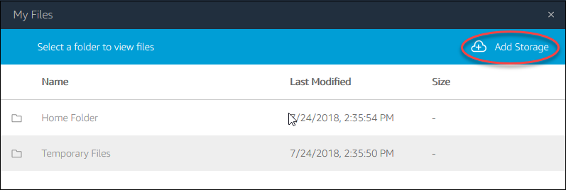
Then select the Drive and the account you want to use.
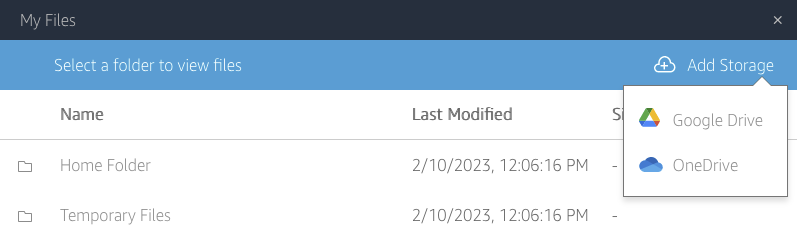
At this point if AppStream has not yet been authorized to access the selected storage, Google Drive or OneDrive may ask you to authorize AppStream to access the storage.
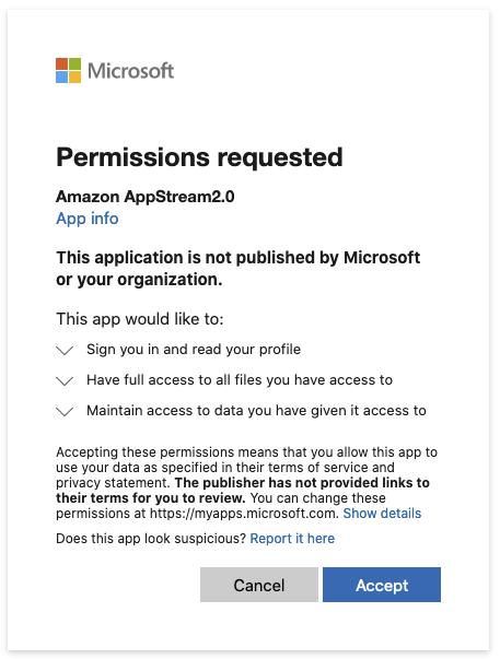
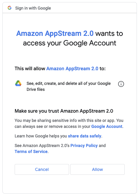
Once you authorized access to your storage, it will appear in the My Files dialog, and the Add Storage button will no longer be available
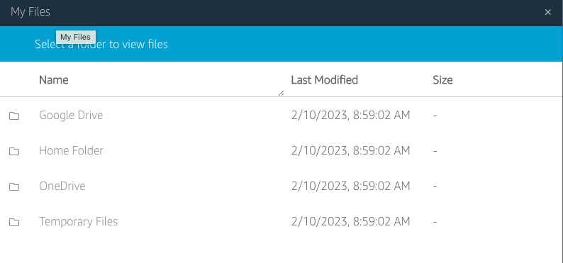
In the applications the new added storage options will look like this:
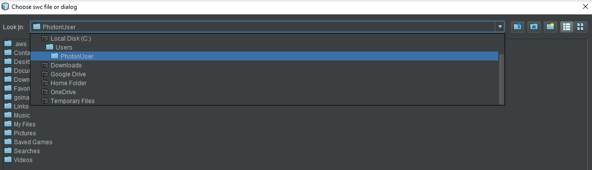
AWS Limits
Most AWS services allow you to setup restrictions on the number of active instances. The default limits, especially for some AppStream resources, such as “Maximum ImageBuilders” for some graphics instances - “stream.graphics.g4dn.xlarge” may be really low (0 in some cases). Connect to AWS console “Service Quotas” service and increase the limit for in case you see a limit was exceeded error. Typically take a look at the limits setup for your account for EC2, VPC, AppStream, S3. Keep in mind that limits may be different from instance type to instance type for AppStream service, so you may have to adjust the limits based on the AppStream instance type selection.
Deploy HortaCloud services
If this is the first time the application is deployed you will need to create a user login pool. This must be explicitly specified using ‘-u’ flag [See Deploy the user login stack section below]:
npm run deploy -- -u
⚠️ The user pool should only be created once.: including the ‘-u’ flag on a future update or deployment will replace all your users accounts!
After the setup is complete, subsequent deployments and updates to the application can be done by running:
npm run deploy
There are a few steps during the deployment that require manual intervention. The deploy script will indicate when these steps should be taken with a ⚠️ warning message.
The full deployment of the application is done in 3, or 4 steps - if user login stack is deployed too, that run automatically one after the other, with some manual intervention for AppStream builder step (third step outlined below):
Deploy the user login stack - this step is optional and practically is only needed first time the application is deployed. To create the user login stack you need to pass in ‘-u’ flag to the deploy command (
npm run deploy -- -u) which will automatically create a Cognito user pool and the ‘admin’ user and ‘admins’ group. You also have an option to import cognito users from a backup (npm run deploy -- -u \ -r -b janelia-mouselight-demo -f hortacloud/backups/20220511030001/cognito) but in this case you may need to skip the creation of the default admin user and group.Deploy the back-end stacks - this includes the AppStream builder. At the back end deployment the installation process will also create the admin user configured in
ADMIN_USER_EMAIL.Connect to AppStream builder and install the Horta application - This is a semiautomated step that involves copying and running two PowerShell scripts onto the AppStream builder instance.
Deploy the administration stack.
Install the Horta desktop application
For client installation start and connect to the AppStream builder instance then copy the following scripts from this repo to the AppStream instance:
- installcmd.ps1 - installs JDK and the Horta application
- createappimage.ps1 - creates the AppStream image
After you copied or created the scripts:
- Log in to the AWS console and go to https://console.aws.amazon.com/appstream2
- Find your new builder in the “Images > Image Builder” tab
- Click on the image name and open an “Administrator” window by clicking on the “Connect” button.
- Copy the installation scripts from your local machine to AppStream:
- Click on the folder icon at the top left of the window
- Select the
Temporary Filesfolder - Use the
Upload Filesicon to find the files on your machine and upload them.
- Open the powershell by typing “`Power shell” in the search found at the bottom left of the window. This step used to require an “Administrator Power Shell” but now it needs only a regular user power shell and it may actually fail the install if you run it in an Administrator Power Shell.
- Change to the directory where you uploaded the installation scripts, eg:
cd 'C:\Users\ImagebuilderAdmin\My Files\Temporary Files'
- Run the installcmd script to install Horta. <serverName> is the name of the backend EC2 instance, typically it looks like
ip-<ip4 with dashes instead of dots>.ec2.internal. Instructions for locating this are provided as output from the installer script. The Horta client certificate is signed using the ec2 internal name so do not use the actual IP for the <serverName> parameter, because user logins will fail with a certificate error.
installcmd.ps1 <serverName>
This will install the JDK and Horta. The installer will run silently and it will install the Horta application under the C:\apps folder. If it prompts you for the install directory, select C:\apps as the JaneliaWorkstation location.
- Optional - To start Horta for testing, run:
c:\apps\runJaneliaWorkstation.ps1
when prompted, login as the admin user you set in ADMIN_USER_EMAIL (leave the password empty)
Navigate through the menus to make sure Horta is working. Do not create any user accounts at this time as they will get created from the Admin web application.
When testing is finished, close down Horta.
Finalize the creation of the AppStream image, run:
createappimage.ps1
Keep in mind that once you start this step the builder instance begins the snap shotting process and it will not be usable until it completes. After this is completed the AppStream image should be available and the builder will be in a stop state. To use it again you need to start it and then you can connect.
- You can now safely close the AppStream session and return to the AppStream console. There you will see a new image in the image registry with a status of
Pending. - Once the image status has changed to a status of
Availableyou can start the fleet by going to theFleetspage on the AppStream site.- Select your fleet from the list of fleets and then select ‘Start’ from the
Actionmenu.
- Select your fleet from the list of fleets and then select ‘Start’ from the
- At this point the installation script you started on your host machine, should continue to completion.
Customizing the portal URL
By default the application will have a very long url that is not easy to remember, something like:
http://janelia-hortacloudwebapp-janeliahortacloudwebadmi-yefcny29t8n6.s3-website-us-east-1.amazonaws.com/. Follow these instructions to create a shorter domain for use with your installation.
- Register a domain with Route53 or your domain provider.
- The Route53 page in the AWS console has a “Register domain” form.
- Alternative providers can also be used, but it requires a little more work.
- Purchase an SSL certificate for your domain.
- This can be done with AWS Certificate Manager
- or an external certificate provider, often it can be done with the same company that provided your domain registration. Use the “Import a certificate” button to register your certificate with AWS.
- Use the “Create distribution” button on the CloudFront console to attach your registered domain to the s3 bucket that hosts the admin portal.
- the only things that need to be changed from the defaults are
- “Origin domain” - this should be the domain that was originally generated for your admin portal. eg: janelia-hortacloudwebapp-janeliahortacloudwebadmi-yefcny29t8n6.s3-website-us-east-1.amazonaws.com
- “Viewer protocol policy” - Change this to “Redirect HTTP to HTTPS”
- “Custom SSL certificate” - Select the certificate that you registered with AWS Certificate Manager
- Finally, click the “Create distribution” button.
- the only things that need to be changed from the defaults are
Configuring demonstration Hortacloud site
To finish setting up self-registration for a demo Hortacloud site, run the post-deployment script to add a post-confirmation trigger to Cognito to synchronize the self-registered user with the HortaCloud database
npm run post-deploy
Uninstalling HortaCloud services
To completely uninstall the application run:
npm run destroy -- -u
The command will uninstall all stacks including the user logins (Cognito) stack.
Note in the previous system upgrade section that an upgrade typically does not require removing and recreating the user pool stack.
Troubleshooting
Troubleshooting client app installation
If the client app installation fails for any reason, before you attempt the install again you must remove everything that was installed by the install script. Uninstall all applications installed with scoop and remove the ‘C:\apps’ folder. To do that run:
scoop uninstall scoop
del c:\apps
When prompted whether you really want to uninstall everything, select “yes” or “all”.
3.1.4 - Backup & Restore
System backup
The system can be configured to take nightly backups. All it is needed is to specify a writeable bucket (HORTA_BACKUP_BUCKET) that will hold the backups. You can also specify the base prefix for the backups using HORTA_BACKUP_FOLDER. If this is not specified the prefix will default to “/hortacloud/backups”.
Currently the backup contains the Cognito users and the Mongo database (user-generated metadata and tracing data). Each backup will be stored in a timestamp (with format “yyyyMMddHHmmss”) folder under the base backup prefix. The location of the backups will be s3://<backup_bucket>/<backup_folder_prefix>/<timestamp>/jacs for the database and s3://<backup_bucket>/<backup_folder_prefix>/<timestamp>/cognito for cognito users.
The backup is configured as a cron job that runs daily at 3 AM local time on the EC2 host on which the backend services run.
System restore
If system backups are available, the sample and tracing data can be restored by specifying a specified backup bucket (HORTA_RESTORE_BUCKET) and prefix (HORTA_RESTORE_FOLDER) which typically was created by the nightly backup job.
3.1.5 - Upgrading
There are two ways to upgrade to a new version of the code: Full Upgrade and Incremental Upgrade.
Full Upgrade
This method backs up all of the data, removes the existing HortaCloud stack, installs a new version from scratch, and restores the data. This is currently the most automated way to upgrade, and requires the least amount of effort.
Backup your data
First, ensure that you have a recent data backup. If you have not configured backups, do that first. For most upgrades, you only need to check if a backup for the JACS Mongo database exists. Typically this is located at s3://<HORTA_BACKUP_BUCKET value>/<HORTA_BACKUP_FOLDER value>/<timestamp>/jacs. If your data is large, you may experience issues with the automatic restore that is performed during the full upgrade. In this case you can perform a manual restore of your data, which is detailed below. To perform a manual backup, you can run the following utility script that will perform a backup.
- <deployment directory, something like /opt/deploy/jacs>/local/run-backup.sh. This script will perform a backup of the database as well as your cognito authentication pool.
- If this script isn’t present, you can run the manage.sh script (usually located in the deployment directory), which will only backup the mongo database
- ./manage.sh mongo-backup <location of mongo jacs backup folder eg., /s3data/backups-bucket/hortacloud/backups/jacs>
Remove HortaCloud environment
To remove the current HortaCloud environment run this command:
npm run destroy
This command will uninstall the frontend and the backend AWS Cloudformation stacks, i.e., Admin, Appstream and JACS stacks, but it will not uninstall Cognito stack, so no user accounts will be removed.
Deploy new version of HortaCloud
The next step is to upgrade the local git repo:
git pull
You should also check out a specific version tag that you want to deploy:
git checkout <version>
In order to restore the database from an existing backup make sure the following properties are set:
NEW_HORTA_ENVIRONMENT=false
HORTA_RESTORE_BUCKET=<backup bucket name>
HORTA_RESTORE_FOLDER="/hortacloud/backups/latest"
HORTA_RESTORE_BUCKET is the name of the backup bucket and HORTA_RESTORE_FOLDER must reference the parent prefix containing the ‘jacs’ folder - the location of the actual mongo backup. Typically the backup job creates a “softlink” - “/hortacloud/backups/latest” so if you simply set the restore folder to that it should pick up the latest backup. If the backup was a manual backup or you need to restore to a previous date set the restore folder to that folder. For example setting HORTA_RESTORE_FOLDER=/hortacloud/backups/20220609030001 will restore the database to the content saved on Jun 9, 2022.
NEW_HORTA_ENVIRONMENT must be set to false so that we don’t try to create another admin user which may clash with the one restored from the backup.
After setting these properties you can proceed with the actual deploy procedure which will only install the backend and the frontend stack (skipping any Cognito installation):
npm run deploy
From here on, this approach is identical with the initial deployment, with the only exception that data and users should already exist once the backend stack is fully deployed.
After you start the deploy command, follow the instructions you see on the screen which will prompt you when you need to setup the AppStream Builder exactly as it is described in the Workstation app-installation section
If somehow you need to recreate the user login accounts because you inadvertently removed the Cognito stack as well (e.g. using -u flag) you can restore all the accounts from a previous backup using the following command:
npm run deploy -- -u -r -b <backup bucket> -f hortacloud/backups/manual-backup/cognito
The folder parameter must point to the actual cognito prefix, where ‘users.json’ and ‘groups.json’ are located
Incremental Upgrade
Incremental approach requires more manual steps, but it does not require any data restore. It basically removes only the frontend stacks, i.e. Appstream and Admin App, and it requires a manual update of the backend stack and the workstation.
The steps for the incremental approach are the following:
Remove only the frontend stacks:
npm run destroy -- -bFrom the AWS console connect to the EC2 instance (
<ORG>-hc-jacs-node-<STAGE>) running the JACS stack using the “Session Manager”. To be more specific, from the EC2 instances page, select the instance<ORG>-hc-jacs-node-<STAGE>and click on the “Connect” button. This will take you to the instance page, and then from there select the “Session Manager’ tab and click the “Connect” button again. The “Connect” button should be enabled - if it’s not there either was a problem with the deployment or there might be a problem with the instance itself.Once connected run the following commands
cd /opt/jacs/deploy
./manage.sh compose down
sudo git pull origin master
sudo git checkout <version>
./manage.sh compose up -d
Start AppStream builder (
<ORG>-hc-image-builder-<STAGE>)Connect as Administrator
Check that ‘reinstallwsonly.ps1’ script is available, in the Admin’s home directory. If not copy it from the application repo or just create it like the other install scripts, (‘installcmd.ps1’ and ‘createappimage.ps1’) were created on the initial deployment.
Run the reinstallwssonly.ps1 script:
.\reinstallwssonly.ps1 <IP of host running JACS stack>The IP of the host running JACS is the same used for initial run of ‘installcmd.ps1’ and it can be found from the AWS console.
Try out the workstation application to make sure it works
C:\apps\runJaneliaWorkstation.ps1Make sure you have the latest ‘createappimage.ps1’ script from the application git repository. If you don’t copy the latest script that supports ‘–skip-registration’ flag.
Start the script for creating the AppStream image but skip the application registration:
.\createappimage.ps1 --skip-registrationReinstall the frontend stacks
npm run deploy -- --skip-vpcIf no changes were made to the code AWS CDK will only update the missing stacks, leaving JACS stack as it was since it practically has not been changed from AWS’ perspective
Restore Your data
If there is a problem with the automatic restoration of your data, you can restore manually using the following process. Be aware that the restoration process can take a long time for large database restoration.
- <deployment directory/local/run-restore.sh. This script will perform a restoration of the database as well as your cognito authentication pool.
- If this script isn’t present, you can run the manage.sh script (usually located in the deployment directory), which will only restore the mongo database
- ./manage.sh mongo-restore <location of mongo jacs backup folder eg., /s3data/backups-bucket/hortacloud/backups/jacs>
3.1.6 - Data Import
Adding the MouseLight Open Data
The MouseLight project at Janelia has made available the complete imagery and neuron tracing annotations for its published data sets on the AWS Open Data Registry.
You can easily make these available in your own HortaCloud instance by creating a Synchronized Folder which points to /s3data/janelia-mouselight-data.
Adding a single volume
A Horta Sample is an object representing a single 3D volume that can be visualized and traced with Horta.
If you already have the HortaKTX format data in your mounted S3 buckets, select File → New → Horta Sample, and then set “Sample Name” to <sampleDirectoryName> and “Path to Render Folder” as /s3data/<bucketName>/<sampleDirectoryName>.
Open the Data Explorer (Window → Core → Data Explorer) and navigate to Home, then “3D RawTile Microscope Samples”, and your sample name. Right-click the sample and choose “Open in Horta”. This will open the Horta Panel and then from the Horta Panel you have options to create a workspace or to open the 2D or the 3D volume viewer.
Converting your data
If your data has not been converted into HortaKTX format, you can use the HortaCloud Data Importer to convert it. This tool supports many common image formats, and can be easily extended in Python to support your favorite format.
3.1.7 - Troubleshooting
No user can login to the workstation
We have seen this behavior if the “/data” volume ran out of space. You can check this by connecting to the EC2 instance running the JACS stack and running df -h /data.
If the disk is full you, you can try to find anything that could be removed but if the limit was reached because the size your data you really have to resize the volume. The steps to resize an EBS volume can be found in the AWS documentation. First run the instructions to increase the size of and EBS volume and then the instructions that make the entire new disk space available to the EC2 instance
If users still cannot use the workstation for tracing, after the /data volume was resized, and there is plenty of disk space available, the reason might be that RabbitMQ failed to start properly, which may happen if RabbitMQ runs out of disk space. Users can also inspect the log from the workstation and look for errors like:
java.lang.IllegalStateException: Message connection could not be opened to host <hostip> after <n> attempts
If this is case check the size of the file /data/db/rabbitmq/jacs/mnesia/rabbit\@jacs-rabbit/msg_stores/vhosts/628WB79CIFDYO9LJI6DKMI09L/recovery.dets If the file exists and its size is 0 then remove the file and restart the entire stack.
3.2 - Bare metal
Warning
This deployment method is no longer supported as we are shifting our development resources to the cloud deployment. You are on your own!The recommended way to deploy HortaCloud is to use Amazon Web Services (AWS), but you can also deploy the Horta services locally on your own client/server machines.
Using Docker Swarm, you can choose to deploy on two or three servers. The primary benefit of using three servers is that the MongoDB cluster will have a complete replica set for high availability.
3.2.1 - Two-server deployment
This document describes the canonical two-server Janelia Workstation deployment for supporting neuron tracing for the MouseLight project at the Janelia Research Campus and other research institutions. This deployment uses Docker Swarm to orchestrate prebuilt containers available on Docker Hub.
Deployment Diagram

Hardware Setup
The JACS backend consists of several services which need to be deployed on server hardware. We have tested the following configuration:
- Two Dell PowerEdge R740XD Servers
- Each server has 40 cores (e.g. Intel Xeon Gold 6148 2.4G)
- Each server has 192 GB of memory
- The hard drives are configured as follows:
- 2 x 200GB SSD in RAID1 - Operating system (/)
- 2 x 960GB SSD in RAID1 - Databases, user preferences, etc. (/opt)
- 12 x 10TB in RAID6 - Image files (/data)
The rest of this guide assumes that you have two server hosts dedicated to deploying this system, which are configured as listed above. They will be referred to as HOST1 and HOST2.
This two-server deployment can support 5-10 concurrent users. We use the following configuration for client machines:
- Dell Precision 5820 Tower
- Minimum of 8 cores (e.g. Intel Xeon W-2145 3.7GHz)
- 128 GB of memory
- Nvidia GTX1080Ti 11GB (reference card, blower fan style)
- Other similar cards will work fine: GTX1070, GTX1080, RTX2080
- Windows 10
Install Oracle Linux 8
The backend software runs on any operating system which supports Docker. However, Oracle Linux is used at Janelia and has been extensively tested with this software. Therefore, we recommend installing the latest version of Oracle Linux 8.
Install Docker
To install Docker and Docker Compose on Oracle Linux 8, follow these instructions.
Setup Docker Swarm
On HOST1, bring up swarm as a manager node:
docker swarm init
On HOST2, copy and paste the output of the previous command to join the swarm as a worker.
docker swarm join --token ...
All further commands should be executed on HOST1, i.e. the master node. One final step is to label the nodes. Each node needs the “jacs=true” label, as well as “jacs_name=nodeX”.
docker node update --label-add jacs_name=node1 $(docker node ls -f "role=manager" --format "{{.ID}}")
docker node update --label-add jacs_name=node2 $(docker node ls -f "role=worker" --format "{{.ID}}")
docker node update --label-add jacs=true $(docker node ls -f "role=manager" --format "{{.ID}}")
docker node update --label-add jacs=true $(docker node ls -f "role=worker" --format "{{.ID}}")
Finally, you can run this command to ensure that both nodes are up and in Ready status:
docker node ls
Download the installer
Download the installer and extract it onto the master node, as follows. VERSION should be set to the latest stable version available on the releases page.
export VERSION=<version_number_here>
cd /opt
sudo mkdir deploy
sudo chown $USER deploy
cd deploy
curl https://codeload.github.com/JaneliaSciComp/jacs-cm/tar.gz/$VERSION | tar xvz
ln -s jacs-cm-$VERSION jacs-cm
cd jacs-cm
Configure The System
Next, create a .env.config file inside the intaller directory. This file defines the environment (usernames, passwords, etc.) You can copy the template to get started:
cp .env.template .env.config
vi .env.config
At minimum, you must customize the following:
- Set
DEPLOYMENTto mouselight. - Ensure that
REDUNDANT_STORAGEandNON_REDUNDANT_STORAGEpoint to the disk mounts you used during the operating system installation. Alternatively, you can make symbolic links so that the default paths point to your mounted disks. - Set
HOST1andHOST2to the two servers you are deploying on. Use fully-qualified hostnames here – they should match the SSL certificate you intend to use. - Fill in all the unset passwords with >8 character passwords. You should only use alphanumeric characters, special characters are not currently supported.
- Generate 32-byte secret keys for JWT_SECRET_KEY, MONGODB_SECRET_KEY, JACS_API_KEY, and JADE_API_KEY.
- If you want to enable automated error reporting from the Workstation client, set
MAIL_SERVERto an SMTP server and port, e.g. smtp.my.org:25.
Deploy Services
Now you can follow the Swarm Deployment instructions to actually deploy the software.
Import Imagery
If you have your own imagery, you will need to convert it before importing.
Each brain image is referred to as a “sample”. You should place each sample in $DATA_DIR/jacsstorage/samples on one of the servers. If you place the sample on the first server, in $DATA_DIR/jacsstorage/samples/<sampleDirectoryName>, then in the Workstation you will refer to the sample as /jade1/<sampleDirectoryName>.
As a side note if you use ’lvDataImport’ service to generate the imagery, the service does not use JADE to persist the data. So if you need the data to be on a storage that is only accessible on certain hosts, JACS must run on that host in order to be able to write the data to the corresponding location. If that is not an option you can generate the data to a temporary location then move it to the intended sample directory.
In the Workstation, select File → New → Horta Sample, and then set “Sample Name” to <sampleDirectoryName> and “Path to Render Folder” as /jade1/<sampleDirectoryName>.
Open the Data Explorer (Window → Core → Data Explorer) and navigate to Home, then “3D RawTile Microscope Samples”, and your sample name. Right-click the sample and choose “Open in Large Volume Viewer”. The 2D imagery should load into the middle panel. You should be able to right-click anywhere on the image and select “Navigate to This Location in Horta (channel 1)”, to load the 3D imagery.
Find More Information
This concludes the MouseLight Workstation installation procedure. Further information on using the tools can be found in the User Manual.
3.2.2 - Three-server deployment
This document describes the full three-server Janelia Workstation deployment for supporting both FlyLight and MouseLight at Janelia Research Campus. This deployment uses Docker Swarm to orchestrate containers available on Docker Hub.
Multiple environments are supported with this deployment:
- prod
- dev
Deployment Diagram

Hardware Setup
This guide assumes that you have three high-end servers which can be dedicated to running Docker Swarm. We use 40-core servers with at least 192 GB of RAM. YMMV.
We’ll refer to the three deployment hosts as HOST1, HOST2, and HOST3.
Note that an additional server or VM is necessary to run the JACS Async Services outside of Docker, if you are planning to submit image processing jobs to an HPC cluster, such as with the Image Processing Pipeline (IPP).
Install Oracle Linux 8
The backend software should run on any operating system which supports Docker. However, Oracle Linux is used at Janelia and has been extensively tested with this software. Therefore, we recommend installing the latest version of Oracle Linux 8. Previously, we used Scientific Linux 7 and that is also known well although it’s no longer supported.
Install Docker
To install Docker and Docker Compose on Oracle Linux 8, follow these instructions.
Setup Docker Swarm
On HOST1, bring up swarm as a manager node, and give it a label:
docker swarm init
On HOST2 and HOST3, copy and paste the output of the previous command to join the swarm as a worker.
docker swarm join --token ...
All further commands should be executed on HOST1, i.e. the master node. One final step is to label the nodes. Each node needs the “jacs=true” label, as well as “jacs_name=nodeX”. You can find out the node ids by running docker node ls.
docker node update --label-add jacs_name=node1 <id of HOST1>
docker node update --label-add jacs_name=node2 <id of HOST2>
docker node update --label-add jacs_name=node3 <id of HOST3>
docker node update --label-add jacs=true <id of HOST1>
docker node update --label-add jacs=true <id of HOST2>
docker node update --label-add jacs=true <id of HOST3>
Download the installer
Download the installer and extract it onto the master node, as follows. VERSION should be set to the latest stable version available on the releases page.
export VERSION=<version_number_here>
cd /opt
sudo mkdir deploy
sudo chown $USER deploy
cd deploy
curl https://codeload.github.com/JaneliaSciComp/jacs-cm/tar.gz/$VERSION | tar xvz
ln -s jacs-cm-$VERSION jacs-cm
cd jacs-cm
Configure The System
Next, create a .env.config file inside the installer directory. This file defines the environment (usernames, passwords, etc.) You can copy the template to get started:
cp .env.template .env.config
vi .env.config
At minimum, you must customize the following:
- Ensure that
REDUNDANT_STORAGEandNON_REDUNDANT_STORAGEpoint to the disk mounts available on the local systems. Alternatively, you can make symbolic links so that the default paths point to your mounted disks. - Set
HOST1,HOST2, andHOST3to the servers you are deploying on. Use fully-qualified hostnames here – they should match the SSL certificate you intend to use. Do not use localhost or the loopback address (127.0.0.1). If you don’t have a DNS name for the hosts, use the host’s IP address. - Fill in all the unset passwords with >8 character passwords. You should only use alphanumeric characters, special characters are not currently supported.
- Generate 32-byte secret keys for JWT_SECRET_KEY, MONGODB_SECRET_KEY and JADE_API_KEY. If JADE_API_KEY is not set jacs-sync service will not be able to register any Mouselight samples.
- Set
JADE_AGENT_VOLUMESto the volumes that you want to be created when you start the system - typicallyjade1,jade2, but these really depend on the volumes that you you setup in your jade service configuration.
Enable Databases (optional)
Currently, Janelia runs MongoDB outside of the Swarm, so they are commented out in the deployment. If you’d like to run the databases as part of the swarm, edit the yaml files under ./deployments/jacs/ and uncomment the databases.
Deploy Services
Now you can follow the Swarm Deployment instructions to actually deploy the software.
Deploy ELK for monitoring
To deploy an ELK stack for monitoring follow ELK Deployment.
Find More Information
This concludes the MouseLight Workstation installation procedure. Further information on using the tools can be found in the User Manual.
3.2.3 - Installing Docker
To install Docker on a server running Oracle Linux 8, some special configuration is needed. Much of this comes from the official documentation.
Prerequisites
First, make sure that Docker isn’t already installed:
yum list installed | grep docker
Remove any existing installations before proceeding.
Ensure that /opt (or whatever disk is to be used for Docker data) is formatted with the d_type option. You can find out like this:
$ xfs_info /opt
meta-data=/dev/mapper/vg0-lv_opt isize=512    agcount=4, agsize=5701632 blks
         =                       sectsz=4096  attr=2, projid32bit=1
         =                       crc=1        finobt=0 spinodes=0
data     =                       bsize=4096   blocks=22806528, imaxpct=25
         =                       sunit=0      swidth=0 blks
naming   =version 2              bsize=4096   ascii-ci=0 ftype=1
log      =internal               bsize=4096   blocks=11136, version=2
         =                       sectsz=4096  sunit=1 blks, lazy-count=1
realtime =none                   extsz=4096   blocks=0, rtextents=0
If the above says ftype=0, then the filesystem will need to be recreated (reference).
Installing Docker
sudo yum install -y yum-utils
sudo yum-config-manager --add-repo https://download.docker.com/linux/centos/docker-ce.repo
sudo yum install -y docker-ce
If this fails with error messages like package containerd.io-1.4.3-3.2.el8.x86_64 conflicts with runc provided by runc then you may have conflicting packages installed already. Try removing them like this:
sudo yum erase podman buildah
Post Install Configuration
To avoid running out of space on the root partition, you should configure docker to point to /opt/docker (reference):
sudo mkdir -p /opt/docker
sudo chown root:root /opt/docker
sudo chmod 701 /opt/docker
Next, configure Docker to use the overlay2 storage driver (reference).
Create a file at /etc/docker/daemon.json with this content:
{
  "data-root": "/opt/docker",
  "storage-driver": "overlay2"
}
You should also create a local user called “docker-nobody” with UID 4444, which can be used for running containers without root.
sudo groupadd -g 4444 docker-nobody
sudo useradd --uid 4444 --gid 4444 --shell /sbin/nologin docker-nobody
Finally, you can start Docker:
sudo systemctl enable docker
sudo systemctl start docker
Installing Docker Compose
You’ll also need to install the Docker Compose executable:
sudo curl -L "https://github.com/docker/compose/releases/download/1.23.2/docker-compose-$(uname -s)-$(uname -m)" -o /usr/local/bin/docker-compose
sudo chmod +x /usr/local/bin/docker-compose
Note that there are newer versions of the Docker Compose, but they have bugs that prevent them from working with our scripts. Please use the version above to ensure compatibility.
3.2.4 - Deploying JACS
This document assumes that you have downloaded and configured the installer according to one of the deployment guides.
The following steps are common to all Docker Swarm deployments of the Workstation.
Initialize Filesystems
The first step is to initialize the filesystems on all your Swarm systems. On each server, ensure that your REDUNDANT_STORAGE (default: /opt/jacs), NON_REDUNDANT_STORAGE (default: /data) directories exist and can be written to by your UNAME:GNAME user (default: docker-nobody).
Then, run the Swarm-based initialization procedure from HOST1:
./manage.sh init-filesystems
You can manually edit the files found in CONFIG_DIR to further customize the installation.
Once the initialization completes you can just run:
./manage.sh stop
Also it is a good idea to stop the initialization stack if anything goes wrong before you try it again.
SSL Certificates
At this point, it is strongly recommended is to replace the self-signed certificates in $CONFIG_DIR/certs/* on each server with your own certificates signed by a Certificate Authority:
. .env
sudo cp /path/to/your/certs/cert.{crt,key} $CONFIG_DIR/certs/
sudo chown docker-nobody:docker-nobody $CONFIG_DIR/certs/*
If you continue with the self-signed certificates, you will need to set up the trust chain for them later.
External Authentication
The JACS system has its own self-contained authentication system, and can manage users and passwords internally.
If you’d prefer that users authenticate against your existing LDAP or ActiveDirectory server, edit $CONFIG_DIR/jacs-sync/jacs.properties and add these properties:
LDAP.URL=
LDAP.SearchBase=
LDAP.SearchFilter=
LDAP.BindDN=
LDAP.BindCredentials=
The URL should point to your authentication server. The SearchBase is part of a distinguished name to search, something like “ou=People,dc=yourorg,dc=org”. The SearchFilter is the attribute to search on, something like “(cn={{username}})”. BindDN and BindCredentials defines the distinguished name and password for a service user that can access user information like full names and emails.
Start All Containers
Next, start up all of the service containers. The parameter to the start command specifies the environment to use. The dev environment uses containers tagged as latest and updates them automatically when they change. The prod deployment uses a frozen set of production versions. When in doubt, use the prod deployment:
./manage.sh start
It may take a minute for the containers to spin up. You can monitor the progress with this command:
./manage.sh status
At this stage, some of the services may not start because they depend on the databases. The next step will take care of that.
Initialize Databases
Now you are ready to initalize the databases:
./manage.sh init-databases
It’s normal to see the “Unable to reach primary for set rsJacs” error repeated until the Mongo replica set converges on healthiness. After a few seconds, you should see a message “Databases have been initialized” and the process will exit successfully.
You can validate the databases as follows:
- Verify that you can connect to the Mongo instance using
./manage.sh mongo, and runshow tables - Connect to the RabbitMQ server at http://HOST1:15672 and log in with your
RABBITMQ_USER/RABBITMQ_PASSWORD
Restart Services
Bounce the stack so that everything reconnects to the databases:
./manage.sh stop
./manage.sh start
Now you shoult wait for all the services to start. You can continue to monitor the progress with this command:
./manage.sh status
If any container failed to start up, it will show up with “0/N” replicas, and it will need to be investigated before moving further. You can view the corresponding error by specifying the swarm service name, as reported by the status command. For example, if jacs_jade-agent2 fails to start, you would type:
./manage.sh status jacs_jade-agent2
Verify Functionality
You can verify the Authentication Service is working as follows:
./manage.sh login
You should be able to log in with the default admin account (root/root), or any LDAP/AD account if you’ve configured external authentication. This will return a JWT that can be used on subsequent requests.
If you run into any problems, these troubleshooting tips may help.
Manage Services
As long as your Docker daemon is configured to restart on boot, all of the Swarm services will also restart automatically when the server is rebooted.
If you want to remove all the services from the Swarm and do a clean restart of everything, you can use this command:
./manage.sh stop
To pull and redeploy the latest image for a single service, e.g. workstation-site:
./manage.sh restart jacs_workstation-site
Configure Crontabs
The following crontab entries should be configured in order to perform periodic maintenance automatically. It’s easiest to install the crontabs on the docker-nobody account:
sudo crontab -u docker-nobody -e
Database maintenance refreshes indexes and updates entities permissions:
0 2 * * * /opt/deploy/jacs-cm/manage.sh dbMaintenance group:admin -refreshIndexes -refreshPermissions
SOLR index refresh (if using SOLR):
0 3 * * * /opt/deploy/jacs-cm/manage.sh rebuildSolrIndex
Database backups (if using containerized databases):
0 4 * * * /opt/deploy/jacs-cm/manage.sh backup mongo
Install The Workstation Client
Now that the services are all running, you can navigate to https://HOST1 in a web browser on your client machine, and download the Workstation client. Follow the installer wizard, using the default options, then launch the Workstation.
If you are using the default self-signed certificate, you will need to take some extra steps to install it on the client.
If you are using LDAP/AD integration, you should be able to log in with your normal user/password. If you are using the Workstation’s internal user management, you must first login as user root (password: root), and then select Window → Core → Administrative GUI from the menus. Click “View Users”, then “New User” and create your first user. Add the user to all of the relevant groups, including MouseLight.
Optional: Adding NFS Storage
If you have data on NFS, and those NFS drives can be mounted on the MouseLight hosts, that data can be made available to the Workstation.
First, create a file at deployments/mouselight/docker-swarm.prod.yml which looks like this:
version: '3.7'
services:
  jade-agent1:
    volumes:
      - /path/to/your/nfs:/path/to/your/nfs:ro,shared
  jade-agent2:
    volumes:
      - /path/to/your/nfs:/path/to/your/nfs:ro,shared
This will expose the path to both JADE agent containers. Now you need to configure the JADE agents to serve this data. On both hosts, edit /opt/jacs/config/jade/config.properties and add the following:
StorageVolume.mouseLightNFS.RootDir=/path/to/your/nfs
StorageVolume.mouseLightNFS.VirtualPath=/path/to/your/nfs
StorageVolume.mouseLightNFS.Shared=true
StorageVolume.mouseLightNFS.Tags=mousebrain,light
StorageVolume.mouseLightNFS.VolumePermissions=READ
You can use any name you want instead of mouseLightNFS. Then you should add this name to StorageAgent.BootstrappedVolumes:
StorageAgent.BootstrappedVolumes=jade1,mouseLightNFS
You will need to bounce the service stack to pick up these changes.
3.2.5 - Deploying ELK
Currently ELK is only available in a swarm deployment because of how the ELK stack is configured.
Most of the set up necessary for ELK - configuration files and/or data directories - is already done as part of filesystem initialization performed while executing:
./manage.sh init-filesystems
The current ELK data directories are created on /data/ directory so this directory must exist.
One manual step is to set the vm.max_map_count value required for running elasticsearch. This is done by adding vm.max_map_count=262144 line to /etc/sysctl.conf and then run sysctl -p (typically this must be done as root)
After that deploying the elk stack for monitoring the application only requires starting with:
./manage.sh start-elk
The command to stop the monitoring is:
./manage.sh stop-elk
Import data from an old stack
To import data from an old stack the old stack nodes must be whitelisted in the ELK_WHITELIST environment variable so that they can be accessible to the current cluster for importing indexes.
Some useful elasticsearch endpoints:
- List available indices
curl http://<escoordinator>:9200/_cat/indices
- Import an index from a remote cluster:
#!/bin/bash

remoteost=$1
indexName=$2

curl -H 'Content-Type: application/json' -X POST http://e03u08.int.janelia.org:9200/_reindex -d "{
    \"source\": {
        \"remote\": {
            \"host\": \"http://${remoteHost}:9200\"
        },
        \"index\": \"${indexName}\",
        \"query\": {
            \"match_all\": {}
        }
    },
    \"dest\": {
        \"index\": \"${indexName}\"
    }
}"
- Export kibana objects
Here’s an example to export kibana visualizations but the command is identical for any one of [config, index-pattern, visualization, search, dashboard, url] - just set the appropriate type
curl http://<oldkibanahost>:5601/api/saved_objects/_export -H 'kbn-xsrf: true' \
     -H 'Content-Type: application/json' \
     -d '{"type": "visualization" }' > local/kibana-visualizations.ndjson
- To import
Use the file generated by the above export command and run
curl -X POST http://e03u06.int.janelia.org:5601/api/saved_objects/_import \
    -H 'kbn-xsrf: true' \
    --form file=@local/kibana-visualizations.ndjson
3.2.6 - Self-signed Certificates
A self-signed certificate is automatically generated during the init-filesystem step of a jacs-cm installation. For production use, it is recommended that you replace this certificate with a real one. The self-signed certificate is less secure, and it requires some extra steps to get working.
In order to connect to https://HOST1, you need to accept the certificate in the browser. This differs by browser.
Then, in order to allow the Workstation to accept the certificate, it needs to be added to Java’s keystore. For this, you will need the certificate on the desktop computer where you are running the Workstation. You can either export it from the browser, or copy it over from the server. On the server, it is located in $CONFIG_DIR/certs/cert.crt. Once you have the certificate, you can import it using Java’s keytool.
Windows
On Windows, click Start and type “cmd” to find the Command Prompt, then right-click it and select “Run as administrator”. You need to find out where your JVM is installed by looking under C:\Program Files\Zulu. Then, import the certificate. Here it’s assumed the cert was saved to the current working directory:
C:\> "C:\Program Files\Zulu\zulu-8\bin\keytool.exe" -import -alias mouse1selfcert -file cert.crt -keystore "C:\Program Files\Zulu\zulu-8\jre\lib\security\cacerts" -keypass changeit -storepass changeit
The alias should be a descriptive name that will be used later if you want to remove or view the certificate. The password for the JVM keystore is actually “changeit”, so don’t change the keypass or storepass values above.
Mac or Linux
First, you need to know where the JVM is located. You can use the same method that the Workstation uses to locate the JVM. This ensures you are modifying the correct one. Open a Terminal and type:
export JDK_HOME=`/usr/libexec/java_home -v 1.8`
Now you can import the certificate into the keystore. Here it’s assumed the cert was saved to the desktop:
sudo keytool -import -v -trustcacerts -alias mouse1 -file ~/Desktop/cert.crt -keystore $JDK_HOME/jre/lib/security/cacerts -keypass changeit -storepass changeit
The alias should be a descriptive name that will be used later if you want to remove or view the certificate. The password for the JVM keystore is actually “changeit”, so don’t change the keypass or storepass values above.
3.2.7 - Storage volumes
The Workstation/JACS system relies on JADE for its storage API.
Adding a new Storage Volume
Add bootstrap to the JADE configuration
On HOST1, edit /opt/jacs/config/jade/config.properties and add a block for your new volume, for example:
StorageVolume.s3data.RootDir=/s3data
StorageVolume.s3data.VirtualPath=/s3jade
StorageVolume.s3data.Shared=true
StorageVolume.s3data.Tags=aws,cloud
StorageVolume.s3data.VolumePermissions=READ,WRITE,DELETE
The properties configure the volume as follows:
- RootDir: defines the actual path to the data on disk
- VirtualPath: optionally defines a virtual path which is mapped to the actual path
- Shared: true if the volume should be accessible to all volumes
- Tags: tags used by applications to find appropriate volumes
- VolumePermissions: list of operations that JADE can execute (READ,WRITE,DELETE)
Also add your volume to StorageAgent.BootstrappedVolumes, so that it will be created the next time the service is restarted.
Mount the path into the containers
Edit the compose/swarm files for your deployment and mount the volume path as a Docker volume. For example, if your DEPLOYMENT is jacs, and STAGE is dev, you must edit these two files:
deployments/jacs/docker-compose.dev.yml
deployments/jacs/docker-swarm.dev.yml
You should add your volume for all services jade-agent<N> which you want to service that volume.
For example:
  jade-agent1:
    volumes:
      - /data/s3data:/s3data:shared
Restart the stack after making the changes above and the volume will be created when the JADE worker starts.
Host-specific Volumes
By default, all JADE agents are configured to serve all volumes in the database. You can use StorageAgent.ServedVolumes to control which volumes are served by which hosts.
3.2.8 - Data import
In principle, any 3d volumetric data can be imported into the MouseLight Workstation. At this moment we only provide some very basic tools for converting only TIFF format images into the expected format on disk. Another limitation of the current tools is that the entire volume must be in a single tiff file (per channel)
The imagery for MouseLight Workstation is a directory containing TIFF and KTX images organized into octrees. JACS compute includes a a service that can generate the octree data from a single volume TIFF file. If there is more than 1 channel, the channels are numbered 0 .. n-1 and each channel is expected to be in its own file. For example if you have 2 channels you would have two tiff files:
/path/to/volume/volume.0.tiff
/path/to/volume/volume.1.tiff
The import service requires docker or singularity installed because the actual conversion services are packaged in two docker containers - one that generates a TIFF octree and the other one that takes the TIFF octree and converts the octant channel images into the correspomding ktx blocks.
Currently pre-built containers for tiff octree tool and ktx tool are only available at Janelia’s internal registry, but the containers build files are available at https://github.com/JaneliaSciComp/jacs-tools-docker.git in the ’tiff_octree’ and ‘ktx_octree’ subdirectories, respectively. KTX tool container can also be built from https://github.com/JaneliaSciComp/pyktx.git.
Generating the sample octree requires only a JACS Async service call which is a simple HTTP REST call that can be done using curl or Postman. This service can also be invoked from the JACS dashboard http://api-gateway-host:8080 by going to the “Services List” after Login and selecting “lvDataImport”. The dashboard should also offer a brief description of each argument.
curl invocation to run the service with singularity (this is the JACS default):
curl -X POST \
  https://api-gateway-host/SCSW/JACS2AsyncServices/v2/async-services/lvDataImport \
  -H 'Accept: application/json' \
  -H 'Content-Type: application/json' \
  -H 'Authorization: Bearer Your_Token' \
  -d '{
        "args": [
                "-containerProcessor", "singularity",
                "-inputDir", "/path/to/volumeData",
                "-inputFilenamePattern", "test.{channel}.tif",
                "-outputDir", "/path/to/lvv/sampleData",
                "-channels", "0,1",
                "-levels", "4",
                "-voxelSize", "1,1,1",
                "-subtreeLengthForSubjobSplitting", 2,
                "-tiffOctreeContainerImage", "docker://registry.int.janelia.org/jacs-scripts/octree:1.0",
                "-ktxOctreeContainerImage", "docker://registry.int.janelia.org/jacs-scripts/pyktx:1.0"
        ],
 "resources": {
 }
}
'
curl invocation to run the service with docker:
curl -X POST \
  https://api-gateway-host/SCSW/JACS2AsyncServices/v2/lvDataImport \
  -H 'Accept: application/json' \
  -H 'Content-Type: application/json' \
  -H 'Authorization: Bearer Your_Token' \
  -d '{
 "args": [
  "-containerProcessor", "docker",
  "-inputDir", "/path/to/volumeData",
                "-inputFilenamePattern", "default.{channel}.tif",
  "-outputDir", "/path/to/lvv/sampleData",
  "-channels", "0",
  "-levels", "3",
  "-voxelSize", "1,1,1",
  "-subtreeLengthForSubjobSplitting", 3,
  "-tiffOctreeContainerImage", "registry.int.janelia.org/jacs-scripts/octree:1.0",
  "-ktxOctreeContainerImage", "registry.int.janelia.org/jacs-scripts/pyktx:1.0"
 ],
 "resources": {
 }
}
'
Arguments description
- containerProcessor - which container runtime to use docker or singularity
- inputDir - path to original volume data
- inputFileNamePattern - original tiff name. Notice that if you have multiple channels and the channel is anywhere in the name you can use
{channel}which will be replaced with the actual channel number. - outputDir - where the octree will be generated - typically this is the sample data directory that will be imported in the workstation
- channels - specifies a list of all available channels, e.g. ‘0,1’ if there are two channels or ‘0’ if there is only 1 channel.
- levels - the number of octree levels. This is left up to the user and the service will not try to figure out the optimum value for the number of octree levels.
- voxelSize - specifies the voxel size in um.
- tiffOctreeContainerImage - tiff octree container image. Not that the format is slightly different for specifying the image name if docker is used or if singularity is used. Since singularity supports docker images, if singularity runtime is used you need to explictily specify that the image is a docker image.
- ktxOctreeContainerImage - ktx octree container image. See above regarding the format based on container processor type.
- subtreeLengthForSubjobSplitting - this parameter applies only for the ktx processor and it tells the service how to split the job and it has a default value of 5. The conversion process typically starts at a certain node and it performs tiff to ktx conversion for a specified number of levels. If you start a process at the root and convert all levels the job may take a while so if you want you have the option to parallelize it by going only for a limited number of levels from the root and start new jobs from all nodes at the level equal with the subtree depth. For example if you have 8 levels and you set
subtreeLengthForSubjobSplittingto3then KTX conversion will start1 + 8^3 + 8^6 = 1 + 512 + 262144 = 262657jobs with the following parameters:"" 3, "111" 3, "112" 3, ..., "118" 3, ..., "888" 3, ..., "111111" 3, ..., "888888" 3If you leave the default (subtreeLengthForSubjobSplitting=5) then the KTX conversion will start only1 + 8^5 = 32769jobs ("11111" 5, ..., "88888" 5)
Note that the service invocation requires authentication so before you invoke it, you need to obtain an JWS token from the authentication service - see the Verify Functionality section on this page.
3.2.9 - Troubleshooting
Docker
These are some useful commands for troubleshooting Docker:
View logs for Docker daemon
sudo journalctl -fu docker
Restart the Docker daemon
sudo systemctl restart docker
Remove all Docker objects, including unused containers/networks/etc.
sudo docker system prune -a
Swarm GUI
If you would like to see the Swarm’s status in a web-based GUI, we recommend installing Swarmpit. It’s a single command to deploy, and it works well with the JACS stack.
Common issues
config variable not set
If you see a lot of errors or warnings similar to the ones below, first check that the .env file was generated correctly - it should have all environment variables from .env.config, present and set. If it is not just remove it and try the commands again. It is possible that you may have run a command like ./manage.sh init-filesystems before the swarm cluster was available.
WARN[0000] The "CONFIG_DIR" variable is not set. Defaulting to a blank string.
WARN[0000] The "DATA_DIR" variable is not set. Defaulting to a blank string.
WARN[0000] The "DB_DIR" variable is not set. Defaulting to a blank string.
WARN[0000] The "BACKUPS_DIR" variable is not set. Defaulting to a blank string.
WARN[0000] The "CERT_SUBJ" variable is not set. Defaulting to a blank string.
WARN[0000] The "DEPLOYMENT" variable is not set. Defaulting to a blank string.
WARN[0000] The "MONGODB_SECRET_KEY" variable is not set. Defaulting to a blank string.
WARN[0000] The "API_GATEWAY_EXPOSED_HOST" variable is not set. Defaulting to a blank string.
WARN[0000] The "RABBITMQ_EXPOSED_HOST" variable is not set. Defaulting to a blank string.
WARN[0000] The "RABBITMQ_USER" variable is not set. Defaulting to a blank string.
WARN[0000] The "RABBITMQ_PASSWORD" variable is not set. Defaulting to a blank string.
WARN[0000] The "MAIL_SERVER" variable is not set. Defaulting to a blank string.
WARN[0000] The "NAMESPACE" variable is not set. Defaulting to a blank string.
WARN[0000] The "REDUNDANT_STORAGE" variable is not set. Defaulting to a blank string.
WARN[0000] The "REDUNDANT_STORAGE" variable is not set. Defaulting to a blank string.
WARN[0000] The "NON_REDUNDANT_STORAGE" variable is not set. Defaulting to a blank string.
WARN[0000] The "NON_REDUNDANT_STORAGE" variable is not set. Defaulting to a blank string.
“network not found”
If you see an intermittent error like this, just retry the command again:
failed to create service jacs-cm_jacs-sync: Error response from daemon: network jacs-cm_jacs-net not found
bind errors during init-filesystems
If during init-filesystems you see an error that the config folder could not be bound on a particular node of the swarm cluster, make sure you did not forget to create the config and db directories on each node that is part of the swarm. The directories must exist in order for docker to be able to mount the corresponding volumes.
After you created all folders if you already ran ./manage.sh init-filesystems and it failed before you run it again stop it using
./manage.sh stop
and then you can try to re-run it
RESTful services
You can access the RESTful services from the command line. Obtain a JWT token like this:
./manage.sh login
The default admin account is called “root” with password “root” for deployments with self-contained authentication.
Now you can access any of the RESTful APIs on the gateway, for instance:
export TOKEN=<enter token here>
curl -k --request GET --url https://${API_GATEWAY_EXPOSED_HOST}/SCSW/JACS2AsyncServices/v2/services/metadata --header "Content-Type: application/json" --header "Authorization: Bearer $TOKEN"
4 - Developer's guide
We are in the process of writing this documentation.
4.1 - Getting started
4.2 - Single server deployment

This document describes a Janelia Workstation deployment intended for setting up a personal development environment. Unlike the canonical distributed deployments which use Docker Swarm, this deployment uses Docker Compose to orchestrate the services on a single server.
Note that this deployment does not build and serve the Workstation client installers, although that could certainly be added in cases where those pieces need to be developed and tested. In most cases, however, it is expected that this server-side deployment be paired with a development client built and run directly from IntelliJ or NetBeans.
System Setup
This deployment should work on any system where Docker is supported. Currently, it has only been tested on Scientific Linux 7 and macOS Mojave.
To install Docker and Docker Compose on Oracle Linux 8, follow these instructions.
Clone This Repo
Begin by cloning this repo:
git clone https://github.com/JaneliaSciComp/jacs-cm.git
cd jacs-cm
Configure The System
Next, create a .env.config file inside the jacs-cm directory. This file defines the environment (usernames, passwords, etc.) You can copy the template to get started:
cp .env.template .env.config
vi .env.config
At minimum, you must customize the following:
- Configured the
UNAMEandGNAMEto your liking. Ideally, these should be your username and primary group. - Setup
REDUNDANT_STORAGEandNON_REDUNDANT_STORAGEto point to directories accessible byUNAME:GNAME. If you want to use the defaults, you may need to create these directories and set the permissions yourself. - Set
HOST1to the hostname you are deploying on. If possible, use a fully-qualified hostname – it should match the SSL certificate you intend to use. - Fill in all the unset passwords with >8 character passwords. You should only use alphanumeric characters, special characters are not currently supported.
- Generate 32-byte secret keys for JWT_SECRET_KEY and MONGODB_SECRET_KEY.
Enable Databases (optional)
Currently, Janelia runs MongoDB outside of the Swarm, so they are commented out in the deployment. If you’d like to run the databases as part of the swarm, edit the yaml files under ./deployments/jacs/ and uncomment the databases.
Initialize Filesystems
The first step is to initialize the filesystem. Ensure that your REDUNDANT_STORAGE (default: /opt/jacs), NON_REDUNDANT_STORAGE (default: /data) directories exist and can be written to by your UNAME:GNAME user (default: docker-nobody).
If you are using Docker for Mac, you’ll need to take the additional step of configuring share paths at Docker -> Preferences… -> File Sharing. Add both REDUNDANT_STORAGE and NON_REDUNDANT_STORAGE and then click “Apply & Restart” to save your changes.
Next, run the filesystem initialization procedure:
./manage.sh init-local-filesystem
You should see output about directories being created and initialized. If there are any errors, they need to be resolved before moving further.
Once the initialization is complete, you can manually edit the files found in CONFIG_DIR. You can use these configuration files to customize much of the JACS environment.
SSL Certificates
At this point, it is strongly recommended is to replace the self-signed certificates in CONFIG_DIR/certs/* with your own certificates signed by a Certificate Authority:
sudo cp /path/to/your/certs/cert.{crt,key} $CONFIG_DIR/certs/
sudo chown docker-nobody:docker-nobody $CONFIG_DIR/certs/*
If you use self-signed certificates, you will need to set up the trust chain for them later.
External Authentication
The JACS system has its own self-contained authentication system, and can manage users and passwords internally.
If you’d prefer that users authenticate against your existing LDAP or ActiveDirectory server, edit $CONFIG_DIR/jacs-sync/jacs.properties and add these properties:
LDAP.URL=
LDAP.SearchBase=
LDAP.SearchFilter=
LDAP.BindDN=
LDAP.BindCredentials=
The URL should point to your authentication server. The SearchBase is part of a distinguished name to search, something like “ou=People,dc=yourorg,dc=org”. The SearchFilter is the attribute to search on, something like “(cn={{username}})”. BindDN and BindCredentials defines the distinguished name and password for a service user that can access user information like full names and emails.
Start All Containers
Now you can bring up all of the application containers:
./manage.sh compose up -d
You can monitor the progress with this command:
./manage.sh compose ps
Initialize Databases
If you are running your own databases, you will need to initalize them now:
./manage.sh init-databases
Verify Functionality
You can verify the Authentication Service is working as follows:
./manage.sh login
You should be able to log in with the default admin account (root/root), or any LDAP/AD account if you’ve configured external authentication. This will return a JWT that can be used on subsequent requests.·
If you run into any problems, these troubleshooting tips may help.
Updating Containers
Containers in this deployment are automatically updated by Watchtower whenever a new one is available with the “latest” tag. To update the deployment, simply build and push a new container to the configured registry.
Stop All Containers
To stop all containers, run this command:
./manage.sh compose down
Build and Run Client
Now you can checkout the Janelia Workstation code base in IntelliJ or NetBeans and run its as per its README.
The client will ask you for the API Gateway URL, which is just http://$HOST1. In order to automatically connect to your standalone gateway instance, you can create a new file at workstation/modules/Core/src/main/resources/my.properties with this content (replacing the variables with the values from your .env.config file):
api.gateway=https://$HOST1
4.3 - System Overview
We are in the process of writing this documentation.
4.3.1 - Persistence
This section covers a basic overview of how Horta persists neurons, workspaces, samples and preferences.
Asynchronous vs synchronous saving
The final persistence store for Horta is in MongoDB, a document database, whether or not the data being saved is asynchronous or synchronous. Most Horta data is saved synchronously; the purpose of the asynchronous saving is to:
Ease the burden on the annotator to constantly save their workShare annotations in realtime with other annotators or machine algorithms working in the same workspace
Persistence flow
All access to MongoDB is wrapped by a RESTful API, jacs-sync, with a number of endpoints for CRUD operations for TmWorkspace, TmSample, and TmNeuronMetadata. The basic class/component diagram is shown below. When a workspace is first loaded, it relies on NeuronModelAdapter to stream in parallel all the neuron annotations for that workspace into the client app. The following initialization steps are performed with the annotation data:
Concurrent map in NeuronModel is populated:LoadWorkspace/Sample events are fired to notify relevant GUI panels to updateSpatial Filters are initialized with vertices (TmGeoAnnotations) from the neurons for snapping and general neighborhood convenience methods

Once the workspace is initialized and the annotator makes a change to a neuron, the entire neuron is serialized into an AMQP message and sent through the NeuronModelAdapter using RabbitMQ. When a client first starts up, it creates a temperorary queue that both publishes to a RabbitMQ topic exchange (ModelUpdates). Another service, jacs-messaging, listens to this exchange using the UpdateProcessor queue, and consumes messages of the exchange. It determines how to process these messages and if it requires persisting the neuron to the db, connects over the REST API to the jacs-sync service to perform the operation.
Once the operation is complete, an acknowledgement/update message is posted on the RabbitMQ fanout exchange, ModelRefresh. If there are any errors, they get posted on the ModelError exchange. All the clients are subscribed the ModelRefresh exchange, so they get notifications on any neuron changes. These are processed as multi-threaded callbacks in RefreshHandler, which filters based off the current workspace and fires update events if the message is relevant.

4.3.2 - Tiled Imagery
Horta 2D
Horta’s 2D and 3D viewer were originally 2 separate visualization packages, so the way that they load tile imagery is quite different. Horta2D was called LVV (Large Volume Viewer) and exclusively loads many 2D slices from a TIFF Octree at a specific resolution to produce a mosaic that fills the window. These 2D slices are retrieved from the jacs-sync REST API based off the current focus on the window.

In the LVV Object Diagram above, the key classes to examine when dealing specifically with the UI are QuadViewUI, TraceMode, AnnotationPanel, SkeletonActorModel, and AnnotationManager. QuadViewUI is the main Swing container for LVV, wrapping the 3D viewer and AnnotationPanel. The AnnotationPanel is the Swing panel on the right of the layout that has all the menu options, neuron filter options and annotation lists for each neuron. TraceMode is the main User EventManager, handling all key presses and mouse clicks. The SkeletonActorModel is the Controller for all the Neuron tracing (anchors/vertexes and directed paths between them).
Horta2D has a different tile-loading mechanism, but shares all other data with Horta3D through TmModelManager, including the current focus location, selection, resolution, voxel-micrometer mapping, etc.
Horta 3D
Horta3D loads 3D tiles as 3D texture-mapped chunks of the type of imagery (KTX, TIFF, MJ2, Zarr) associated with the current workspace/sample. These chunks all inherit from GL3Actor (TetVolumeActor, BrickActor), and are all loaded into a collection that is rendered by NeuronMPRenderer in its VolumeRenderPass. The main JOGL OpenGL window is SceneWindow.
When Horta3D is first loaded, the focus location is initialized from the sample bounding box and center information that is calculated on scene/workspace loading. The top component of Horta3D, NeuronTracerTopComponent, then delegates to the NeuronTileLoader to find the appropriate 3D chunks for that view. The BrickSource objects are used to load 3D voxel data and convert it into a 3D object that can be rendered in the SceneWindow.
In the case of KTX, the TetVolumeActor and KTXBlockLoadRunner work together to queue up a number of 3D chunks for multi-threaded loading based off the zoom resolution and current focus in the SceneWindow. The intent is to load as many chunks are necessary to fill up the viewport.

4.3.3 - Event Handling/Communication
This section briefly covers how information is shared throughout the GUI in Horta
EventBus
To preserve code independence between different modules in Horta, an EventBus from Google is used. This acts likes an internal publish/subscribe framework within the client, allowing methods to listen for certain events to happen. Events are sent asynchronously on the EventBus, so they are managed in a separate thread than the main AWT thread.
In Horta, the EventBus is mainly used to communicate events that concern multiple GUI components. Events that are mostly concerned with communication within a GUI component are still managed using Listeners.
ViewerEventBus is the main wrapper around the eventbus for Horta, and is managed by TmViewerManager.- `Each main component has a Controller class that is the main hub for incoming eventbus messages (eg, PanelController for the Horta Command Center). Messages are then appropriately routed to local GUI components from the controller.
All the eventbus events are listed in the org.janelia.workstation.controller.eventbus package and include events such as SampleCreateEvent, WorkflowEvent, etc. Because events can have inheritance, methods can listen to the super Event class and get notifications on the whole stack of events that inherit from the super class.
4.4 - Contribution guidelines
5 - Support
Janelia Scientific Computing supports HortaCloud as part of our Open Science Software Initiative. As part of the HortaCloud Community Project, we aim to:
- Maintain the code base to ensure long-term stability and usability.
- Serve as the open-source project lead for coordinating and integrating code contributions.
- Create and release new versions of the software as appropriate.
- Receive feedback through direct communication and GitHub Issues, which we try to address as soon as possible. However, we are limited by the amount of funding available through the Open Science Software Initiative as well as potential internal projects with higher priority.
- Host periodic community meetings to discuss user experiences and development updates.
- Provide guidance and advice to users and developers working with HortaCloud.
- Continue to update the documentation as questions are addressed.
To ensure sustainable support and foster a collaborative community, there are certain types of assistance we are not able to provide.
- Guaranteed support within a certain time frame or on-call availability.
- Hands-on changes or troubleshooting directly within users’ environments.
- We may provide guidance, but are not able to carry out direct operations on user systems.
- Suggestions will be provided as GitHub Gists so that they are reusable and can be referenced later.
- Implementation of new features is generally limited to those that align with Janelia’s priorities.
- However, we very much welcome community contributions and are happy to provide guidance for externally driven feature development.
These boundaries help us focus on maintaining a robust, open, and community-driven platform while managing the limited resources of our development team.
Getting Help
If you encounter an issue with the documentation or a bug in the software system, or if you want to suggest a new feature, please create a new issue on GitHub.
6 - Editing the documentation
We use Hugo to format and generate our website, the Docsy theme for styling and site structure, and GitHub Pages to manage the deployment of the site.
Hugo is an open-source static site generator that provides us with templates, content organization in a standard directory structure, and a website generation engine. You write the pages in Markdown (or HTML if you want), and Hugo wraps them up into a website.
All submissions, including submissions by project members, require review. We use GitHub pull requests for this purpose. Consult GitHub Help for more information on using pull requests.
Updating a single page
If you’ve just spotted something you’d like to change while using the docs, Docsy has a shortcut for you:
- Click Edit this page in the top right hand corner of the page.
- If you don’t already have an up to date fork of the project repo, you are prompted to get one - click Fork this repository and propose changes or Update your Fork to get an up to date version of the project to edit. The appropriate page in your fork is displayed in edit mode.
Previewing your changes locally
If you want to run your own local Hugo server to preview your changes as you work:
Follow the instructions to install Hugo. It must be the extended version, which supports SCSS.
Fork the HortaCloud website repo locally:
git clone --recurse-submodules --depth 1 https://github.com/JaneliaSciComp/hortacloud-websiteRun
npm installandhugo serverin the site root directory. By default your site will be available at http://localhost:1313/. Now that you’re serving your site locally, Hugo will watch for changes to the content and automatically refresh your site.Continue with the usual GitHub workflow to edit files, commit them, push the changes up to your fork, and create a pull request.
Creating an issue
If you’ve found a problem in the docs, but you’re not sure how to fix it yourself, please create an issue in the HortaCloud website repo. You can also create an issue about a specific page by clicking the Create Issue button in the top right hand corner of the page.